The Bias-Variance Dilemma

How Complex Should the Model Be?

In Chapter 5 we cracked Chibany’s bento mystery with a Gaussian Mixture Model — but only after we fixed the number of components $K$ by hand. Choosing $K=2$ was not a detail; it was a decision about how complex the model is allowed to be. Pick $K$ too small and the model cannot capture the structure that is really there. Pick it too large and it starts inventing structure out of noise.

That tension — too simple versus too complex — is the single most important idea standing between “a model that fits the data you have” and “a model that predicts data you have not yet seen.” It has a name: the bias-variance dilemma, and it is the subject of this chapter.

To study it cleanly we leave clustering behind for a simpler testbed: fitting a curve to noisy points. Chibany weighs the lunch bento every day and suspects its weight varies smoothly with something measurable — the morning temperature, say. We have a handful of noisy (temperature, weight) readings and want to predict the weight at a new temperature. The model is a polynomial of some degree $d$:

The degree $d$ is our complexity knob — exactly like $K$ was for the mixture. A degree-1 polynomial is a straight line (very rigid); a degree-12 polynomial can wiggle through almost any twelve points (very flexible). Which one should we trust?

We will build the whole testbed as a GenJAX generative model, because it pays an unexpected dividend later: the prior we put on the polynomial coefficients turns out to be the famous regularization trick (ridge regression). Here is the model. The unknown truth is a fixed cubic the model never gets to see; it only ever sees noisy samples of it.

 1
 2
 3
 4
 5
 6
 7
 8
 9
10
11
12
13
14
15
16
17
18
19
20
21
22
23
24
25
26
27
28
29
30
31
32
33
34
35
36
37
38
39
40
41
42
43
44
45
46
47
48
49
50
51

import jax
import jax.numpy as jnp
import numpy as np
from genjax import gen, normal

# The unknown truth: a fixed cubic on [0, 1]. The model NEVER sees this form —
# it only sees noisy samples y = true_f(x) + noise. Whatever error survives
# because our polynomial family cannot match this curve is "bias."
def true_f(x):
    return 1.7 * (x - 0.18) * (x - 0.55) * (x - 0.88) * 5.0

TAU = 3.0      # prior std on each coefficient beta_j  (a wide, vague prior)
SIGMA = 0.25   # observation-noise std: how noisy each measurement is

def design_matrix(x, degree):
    """Rows [1, t, t^2, ..., t^degree] with t = 2x - 1 in [-1, 1].
    Re-centering x keeps the high powers well-conditioned."""
    t = 2.0 * x - 1.0
    return jnp.stack([t ** j for j in range(degree + 1)], axis=-1)

def make_regression_model(x, degree):
    """Factory returning a @gen Bayesian polynomial-regression model.
    `degree` is captured as a Python constant in the closure — a traced
    range(degree) over a model ARGUMENT would raise in GenJAX."""
    Phi = design_matrix(x, degree)          # design matrix, shape (n, degree+1)
    p = degree + 1                          # number of coefficients

    @gen
    def model(tau, sigma):
        beta = normal(jnp.zeros(p), tau) @ "beta"   # one Gaussian prior per coefficient
        mu = Phi @ beta                              # noise-free curve at the inputs
        y = normal(mu, sigma) @ "y"                  # noisy observations
        return y
    return model

# Exercise the model: draw a few candidate curves from the PRIOR — before any
# data — by simulating coefficients and reading them back out of the trace.
key = jax.random.key(0)
grid = jnp.linspace(0.0, 1.0, 200)
prior_model = make_regression_model(grid, degree=6)
Phi_grid6 = design_matrix(grid, 6)

def one_prior_function(k):
    tr = prior_model.simulate(k, (TAU, SIGMA))
    beta = tr.get_choices()["beta"]        # the sampled coefficient vector
    return Phi_grid6 @ beta                 # the smooth curve it implies
prior_funcs = jax.vmap(one_prior_function)(jax.random.split(key, 6))

print("Drew", prior_funcs.shape[0], "candidate functions from the degree-6 prior")
print(f"Their values span roughly [{float(prior_funcs.min()):+.1f}, {float(prior_funcs.max()):+.1f}]"
      " before any data")

Output:

Drew 6 candidate functions from the degree-6 prior
Their values span roughly [-9.5, +14.6] before any data

The prior, with its wide TAU = 3.0, is happy to propose curves swinging across a broad range — it has no opinion yet. Data will pin it down. The question is how much flexibility we should give it.

Underfitting and Overfitting

Let’s draw one noisy dataset from the true cubic and fit it at three degrees: 1 (a line), 3 (matches the truth’s complexity), and 12 (far more flexible than needed). We fit with the posterior mean of the model above — the closed form is the ridge estimator, which Section 5 unpacks; for now treat it as “the best-fit coefficients, gently pulled toward zero by the prior.”

We report two numbers per degree. Training error is the fit’s RMSE on the very points it was trained on. Error vs. truth is its RMSE against the true cubic on a dense grid — the thing we actually care about but, in real life, never get to measure.

 1
 2
 3
 4
 5
 6
 7
 8
 9
10
11
12
13
14
15
16
17
18
19
20
21
22
23
24
25

def ridge_posterior_mean(Phi, y, tau, sigma):
    """Posterior mean of the @gen model above == the ridge estimator:
       beta_hat = (Phi^T Phi + (sigma^2/tau^2) I)^{-1} Phi^T y."""
    p = Phi.shape[-1]
    lam = (sigma ** 2) / (tau ** 2)
    A = Phi.T @ Phi + lam * jnp.eye(p)
    return jnp.linalg.solve(A, Phi.T @ y)

@gen
def observe(mu, sigma):
    """Shared Gaussian likelihood — we draw the noisy dataset THROUGH GenJAX."""
    return normal(mu, sigma) @ "y"

# One noisy dataset of n = 20 points from the TRUE cubic.
n = 20
kx, ko = jax.random.split(jax.random.fold_in(key, 99))
x = jax.random.uniform(kx, (n,))
y = observe.simulate(ko, (true_f(x), SIGMA)).get_retval()

print("degree   train error   error vs. truth")
for d in (1, 3, 12):
    beta_hat = ridge_posterior_mean(design_matrix(x, d), y, TAU, SIGMA)
    train = float(jnp.sqrt(jnp.mean((design_matrix(x, d) @ beta_hat - y) ** 2)))
    truth = float(jnp.sqrt(jnp.mean((design_matrix(grid, d) @ beta_hat - true_f(grid)) ** 2)))
    print(f"  {d:>2}        {train:.3f}          {truth:.3f}")

Output:

degree   train error   error vs. truth
   1        0.287          0.178
   3        0.218          0.055
  12        0.207          0.092

Read the two columns against each other — they tell opposite stories:

• Training error only ever falls as we add capacity (0.287 → 0.218 → 0.207). More flexibility can always fit the points you already have at least as well. Training error is not a safe guide to complexity.
• Error against the truth is U-shaped (0.178 → 0.055 → 0.092). It bottoms out at degree 3 and climbs back up.

Those two regimes have names:

• Underfitting (degree 1): the model is too rigid to represent the truth. A straight line simply cannot bend into a cubic, so it is wrong no matter what data it sees. This is a failure of bias.
• Overfitting (degree 12): the model is flexible enough to capture the truth, but it spends that flexibility chasing the noise in these particular 20 points. Show it a different 20 points and it would draw a very different wiggly curve. This is a failure of variance.
• Just right (degree 3): flexible enough to bend into the cubic, rigid enough to ignore the noise.

The left panel below shows all three fits against the truth and the single dataset. Degree 1 (red) cuts straight through, missing the curve. Degree 3 (green) tracks the truth almost perfectly. Degree 12 (orange) hugs the data points but wobbles between them — and those wobbles are exactly where it goes wrong.

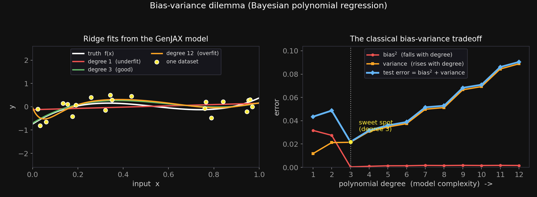
(We will read the right panel in Section 4, once we have defined bias and variance precisely.)

The Bias-Variance Decomposition

Why must error split into “too rigid” and “too jumpy”? Because it provably does. Here is the one piece of math in the chapter, and it is worth seeing once.

Fix a test input $x$. The truth generates its label with noise:

where $f$ is the true function (our cubic), and $\sigma^2$ is the irreducible noise variance — the part of $y$ that nothing about $x$ can explain. Our prediction $\hat{y}(x)$ is itself random, because it was fit on a random training set $D$; train on different data and you get a different $\hat{y}$. Averaging the squared error over both the noise $\varepsilon$ and the random dataset $D$, and writing $\bar{y}(x) = \mathbb{E}_D[\hat{y}(x)]$ for the average prediction across datasets, gives the bias-variance decomposition:

The trick is just add and subtract $\bar{y}(x)$ inside the square and expand; the cross-term vanishes because $\varepsilon$ and $D$ are independent and $\varepsilon$ is mean-zero. The three survivors are:

• Bias $= \bar{y}(x) - f(x)$. How far the average fit lands from the truth. Bias is large when the fitted family is wrong — a line averaging over all possible datasets is still a line, and a line is not a cubic. Bias does not care about any single dataset; it is a property of the model class.
• Variance $= \mathbb{E}_D[(\hat{y}(x) - \bar{y}(x))^2]$. How much the fit jumps around as the dataset changes. Variance is large when the model is flexible enough to mold itself to the particular noise in each dataset.
• Noise $= \sigma^2$. The irreducible floor. No model, however perfect, can predict the coin-flip part of $y$ below $\sigma^2$.

Two of these we control by choosing complexity; the third we are stuck with:

Underfitting is the top-left/bottom-left corner (bias dominates); overfitting is the right column (variance dominates). The art is trading one against the other.

The U-Curve

Let’s measure the trade-off instead of arguing about it. We resample many datasets, fit every one at each degree, and estimate bias and variance directly from the definitions above:

• bias² = average over the grid of $(\text{mean fit} - \text{truth})^2$,
• variance = average over the grid of the per-point variance of the fits across datasets,
• total = bias² + variance (the reducible error; we measure against the noise-free truth, so the $\sigma^2$ floor is not added in here — it would simply shift every row up by the same constant).

 1
 2
 3
 4
 5
 6
 7
 8
 9
10
11
12
13
14
15
16
17
18
19
20
21
22
23
24
25
26
27
28
29
30
31
32
33

def sample_datasets(key, M, n):
    """Draw M independent datasets, sharing them across all degrees so the
    bias/variance curves are comparable. Noise is drawn THROUGH GenJAX."""
    kx, ky = jax.random.split(key)
    X = jax.random.uniform(kx, (M, n))
    mu = true_f(X)
    keys = jax.random.split(ky, M)
    Y = jax.vmap(lambda k, m: observe.simulate(k, (m, SIGMA)).get_retval())(keys, mu)
    return X, Y

def bias_variance_sweep(key, degrees, M=60, n=20, n_grid=200):
    grid = jnp.linspace(0.0, 1.0, n_grid)
    f_grid = true_f(grid)
    X, Y = sample_datasets(key, M, n)
    bias2, variance, total = [], [], []
    for d in degrees:
        Phi_grid = design_matrix(grid, d)
        def fit_eval(x_i, y_i):
            beta_hat = ridge_posterior_mean(design_matrix(x_i, d), y_i, TAU, SIGMA)
            return Phi_grid @ beta_hat              # this dataset's fit, on the grid
        fits = jax.vmap(fit_eval)(X, Y)             # (M, n_grid)
        mean_fit = jnp.mean(fits, axis=0)
        b2 = float(jnp.mean((mean_fit - f_grid) ** 2))   # bias^2
        v = float(jnp.mean(jnp.var(fits, axis=0)))       # variance
        bias2.append(b2); variance.append(v); total.append(b2 + v)
    return np.array(bias2), np.array(variance), np.array(total)

degrees = np.arange(1, 13)
bias2, variance, total = bias_variance_sweep(jax.random.fold_in(key, 2), degrees)
print("degree   bias^2   variance    total")
for d, b, v, tt in zip(degrees, bias2, variance, total):
    print(f"  {d:>2}     {b:.4f}    {v:.4f}    {tt:.4f}")
print("lowest total (test) error at degree", int(degrees[np.argmin(total)]))

Output:

degree   bias^2   variance    total
   1     0.0317    0.0118    0.0435
   2     0.0275    0.0212    0.0487
   3     0.0004    0.0215    0.0218
   4     0.0009    0.0308    0.0317
   5     0.0013    0.0346    0.0360
   6     0.0014    0.0375    0.0389
   7     0.0017    0.0499    0.0515
   8     0.0015    0.0513    0.0528
   9     0.0017    0.0665    0.0682
  10     0.0016    0.0693    0.0708
  11     0.0017    0.0844    0.0861
  12     0.0016    0.0888    0.0904
lowest total (test) error at degree 3

There is the whole story in three columns. Bias² collapses from 0.0317 to 0.0004 the instant the degree reaches 3 — once the polynomial family is rich enough to contain a cubic, the average fit nails the truth, and adding more degrees buys no further bias reduction. Variance climbs steadily, from 0.0118 at degree 1 to 0.0888 at degree 12 — every extra coefficient is one more knob the model can wiggle to chase noise. Their sum is the famous U-curve (the blue line in the right panel of the figure above): falling while bias dominates, flat at the bottom, then rising as variance takes over. The minimum — the sweet spot — sits at degree 3, exactly the complexity of the truth.

Ridge Regression Is a Gaussian Prior

We have been turning one knob — the degree. There is a second, gentler knob hiding in our model, and it is the bridge to a much bigger idea.

Look again at the prior in make_regression_model:

1
2

# (illustrative fragment from make_regression_model above — not run standalone)
beta = normal(jnp.zeros(p), tau) @ "beta"   # beta_j ~ Normal(0, tau)

Each coefficient gets an independent $\text{Normal}(0, \tau)$ prior: a priori, we expect the coefficients to be smallish (near 0), and tau says how small. Now ask what the posterior mean of this model is. The log-posterior is the log-likelihood plus the log-prior:

Maximizing it is the same as minimizing

That second term — a penalty on the size of the coefficients — is exactly ridge regression (also called $L_2$ regularization): “fit the data, but keep the coefficients small.” The penalty strength has a name, $\lambda$, and our derivation just told us what it is:

So the Gaussian prior on the coefficients is the ridge penalty — they are the same object seen from two sides. A statistician writes a penalty $\lambda \lVert\beta\rVert^2$; a Bayesian writes a prior $\beta_j \sim \text{Normal}(0, \tau)$; the math is identical. And $\lambda$ is not a free dial we tune by magic — in the Bayesian view it is dictated by how noisy the data are ($\sigma$) and how large we believe the coefficients to be ($\tau$):

1
2
3
4

lam_default = SIGMA ** 2 / TAU ** 2
print(f"observation noise  sigma = {SIGMA}")
print(f"prior width        tau   = {TAU}")
print(f"=> ridge penalty   lambda = sigma^2 / tau^2 = {lam_default:.5f}")

Output:

observation noise  sigma = 0.25
prior width        tau   = 3.0
=> ridge penalty   lambda = sigma^2 / tau^2 = 0.00694

A tighter prior (small $\tau$) means a larger $\lambda$ — stronger shrinkage, coefficients squeezed harder toward zero, lower variance but higher bias. A looser prior (large $\tau$) means $\lambda \to 0$ — barely any shrinkage, back toward ordinary least squares, higher variance.

But why should shrinking the coefficients toward zero help us predict new data at all? Because noise corrupts only specific data points, while the true signal shows up across all of them. Penalizing large coefficients biases the fit to invest in the directions that help many points (the signal) rather than a few (the noise) — so shrinkage trades a little bias for a large cut in variance, and that is why it generalizes.

Ridge gives us a continuous complexity knob, finer than the integer degree: we can keep a flexible high-degree model but tame its variance with the prior. Section 7 turns that knob and reads off where it leads.

Double Descent

Everything so far says: past the sweet spot, more complexity is strictly worse — variance runs away, test error climbs forever. For most of statistics’ history that was the end of the story. It is also, for very flexible models, wrong.

Push the capacity all the way up to where the model has exactly as many parameters as data points — the interpolation threshold, $p = n$ — and something violent happens: the model can hit every training point exactly, training error is zero, and to do it the fit contorts into wild swings between the points. Test error doesn’t just rise; it explodes. But keep going — give the model more parameters than data points, $p > n$ — and among the infinitely many parameter settings that interpolate the data, the fitting procedure quietly prefers the smallest one (the minimum-norm solution: of all coefficient settings that fit the training data exactly, the one with the smallest $\lVert\beta\rVert_2$). That implicit preference acts like a prior, and test error descends a second time. Two descents, with a spike between them: double descent.

Why does dimension flip the verdict? Picture what the minimum-norm interpolant is forced to do. In one dimension it has essentially a single feature to work with, so to thread every noisy point it must strain that one feature to fit signal and noise at once — and its norm blows up, dragging test error up with it. In high dimensions the picture inverts. With $D = 180$ features but only $n = 20$ points, the fit has a vast space of directions to spread its weight across; the minimum-norm solution can lean on the many directions aligned with the true signal and put almost no weight on the directions that merely capture noise. Its built-in preference for small norm then behaves like a regularizer — the model interpolates the noisy data exactly yet still generalizes well (benign overfitting). That ability to spread thinly is why benign overfitting is a high-dimensional phenomenon: only when there are many directions does “take the smallest interpolant” become a useful bias rather than a desperate stretch of one feature.

This is also why the demo cannot stay with the degree-$d$ polynomials of the earlier sections: a low-degree polynomial offers only a handful of effective directions — far too few for the minimum-norm solution to regularize itself by spreading. To get a genuinely high-dimensional model we switch to $D = 180$ isotropic Gaussian random features, comfortably overparameterized at roughly $9n$ (not a magic number — just safely past the $n = 20$ interpolation threshold).

We sweep capacity $p$ from 1 up to $8n$, fitting the minimum-norm least-squares solution at each, and measure test error against the noise-free signal (so this is bias² + variance, no noise floor):

 1
 2
 3
 4
 5
 6
 7
 8
 9
10
11
12
13
14
15
16
17
18
19
20
21
22
23
24
25
26
27
28
29
30
31
32

def fit_min_norm(Xtr, ytr, n):
    """Minimum-norm least squares.
       p <= n: ordinary normal equations (tiny ridge only for stability).
       p  > n: the minimum-NORM interpolant via the (n x n) Gram matrix —
               of all settings that hit the data exactly, the smallest one."""
    p = Xtr.shape[1]
    if p <= n:
        A = Xtr.T @ Xtr + 1e-8 * np.eye(p)
        return np.linalg.solve(A, Xtr.T @ ytr)
    G = Xtr @ Xtr.T + 1e-8 * np.eye(n)
    return Xtr.T @ np.linalg.solve(G, ytr)

def double_descent(seed=0, n=20, D=180, sigma=0.3, decay=0.9, reps=60, n_test=2500):
    rng = np.random.default_rng(seed)
    theta = decay ** np.arange(D); theta = theta / np.linalg.norm(theta)  # true signal
    Ztest = rng.standard_normal((n_test, D))
    test_signal = Ztest @ theta                       # noise-free test targets
    ps = np.arange(1, 8 * n + 1)
    risk = np.zeros(len(ps))
    for _ in range(reps):
        Ztr = rng.standard_normal((n, D))
        ytr = Ztr @ theta + sigma * rng.standard_normal(n)   # noisy training labels
        for i, p in enumerate(ps):
            beta = fit_min_norm(Ztr[:, :p], ytr, n)          # use the first p features
            risk[i] += np.mean((Ztest[:, :p] @ beta - test_signal) ** 2)
    return ps, risk / reps, n

ps, risk, n = double_descent()
print(f"under-parameterized   p = 1:     test error = {risk[0]:.2f}   (high bias, underfit)")
print(f"the risk curve PEAKS at p = {int(ps[np.argmax(risk)])}   (= n, the interpolation threshold)")
print(f"over-parameterized    p = 8n:    test error = {risk[-1]:.2f}   (second descent)")
print(f"best over-parameterized error  = {risk[ps >= 2 * n].min():.2f}")

Output:

under-parameterized   p = 1:     test error = 0.86   (high bias, underfit)
the risk curve PEAKS at p = 20   (= n, the interpolation threshold)
over-parameterized    p = 8n:    test error = 0.90   (second descent)
best over-parameterized error  = 0.60

The peak sits exactly at $p = n = 20$ — the interpolation threshold — where the test error blows up by more than two orders of magnitude (off the top of the plot below; on the linear scale it reaches the hundreds). To its left is the classical U you already know. To its right, the error falls again and settles back near the floor: the over-parameterized models, despite interpolating noisy data, generalize well. This is benign overfitting — overfitting that does not hurt — and it is why a modern neural network with millions of parameters can fit its training set perfectly and still predict well.

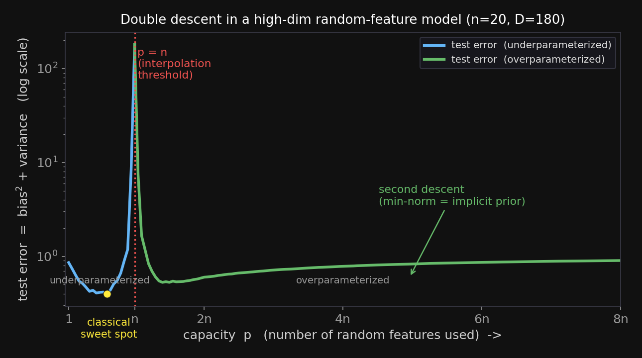
Notice the honest detail in the numbers: the best over-parameterized error (0.60) is good — far below the underfit (0.86) and astronomically below the spike — but it does not beat the classical sweet spot to the left. The second descent rescues you from the spike; it does not, by itself, hand you the best model in the world. For that, we turn the ridge knob.

Explore it yourself

The widget below is the whole chapter in one canvas. In classical view it draws the bias-variance U as you drag the polynomial degree; switch to the double-descent view to push capacity $p$ through the interpolation threshold and watch the spike form and the second descent appear.

What to try: drag degree up and watch the red bias curve fall while the orange variance curve rises; then flip to the double-descent view, push capacity $p$ past $n$ to make the spike erupt, and finally raise the ridge $\lambda$ slider — the spike melts away. If the widget doesn’t load, the two figures above show the same two curves.

Ridge, Honestly — and the Bridge

That melting spike deserves an honest accounting, because it is easy to oversell. Let’s turn the ridge knob from Section 5 properly. We hold the model deliberately over-complex (degree 10, far past the truth’s degree 3) and sweep the penalty $\lambda = \sigma^2/\tau^2$ from almost nothing (huge tau) to very strong (tiny tau), measuring test error each time:

 1
 2
 3
 4
 5
 6
 7
 8
 9
10
11
12
13
14
15
16
17
18
19
20
21

def avg_test_error(key, degree, tau, sigma=SIGMA, M=60, n=20, n_grid=200):
    """Average bias^2 + variance for a fixed degree at prior width tau (penalty
    lambda = sigma^2 / tau^2), over M resampled datasets."""
    grid = jnp.linspace(0.0, 1.0, n_grid)
    f_grid = true_f(grid)
    X, Y = sample_datasets(key, M, n)
    Phi_grid = design_matrix(grid, degree)
    def fit_eval(x_i, y_i):
        beta_hat = ridge_posterior_mean(design_matrix(x_i, degree), y_i, tau, sigma)
        return Phi_grid @ beta_hat
    fits = jax.vmap(fit_eval)(X, Y)
    mean_fit = jnp.mean(fits, axis=0)
    b2 = float(jnp.mean((mean_fit - f_grid) ** 2))
    v = float(jnp.mean(jnp.var(fits, axis=0)))
    return b2 + v

print("  tau     lambda      test error")
for tau in (30.0, 3.0, 1.0, 0.5, 0.2, 0.05):
    lam = SIGMA ** 2 / tau ** 2
    err = avg_test_error(jax.random.fold_in(key, 7), 10, tau)
    print(f" {tau:5.2f}   {lam:8.5f}    {err:.4f}")

Output:

  tau     lambda      test error
 30.00    0.00007    0.9524
  3.00    0.00694    0.0547
  1.00    0.06250    0.0190
  0.50    0.25000    0.0147
  0.20    1.56250    0.0182
  0.05   25.00000    0.0291

Read it top to bottom — it is a U all over again, but now in $\lambda$ rather than in degree:

• Almost no penalty (tau = 30, $\lambda \approx 0.00007$): test error 0.95 — the degree-10 model overfits wildly, pure variance.
• A moderate penalty (tau = 0.5, $\lambda = 0.25$): test error 0.0147 — the lowest of anything we have seen. It is below even the best unregularized degree (degree 3 scored 0.0218 in Section 4). A flexible model with the right shrinkage beats the best rigid model outright.
• Too much penalty (tau = 0.05, $\lambda = 25$): test error climbs back to 0.029 — over-shrinkage squashes the coefficients toward zero and the model underfits again.

So the honest summary of ridge is sharper than “it removes the spike”:

One Question, Three Answers

Step back. Every section of this chapter has been answering the same question — how complex should the model be? — and we have now seen that there is not one answer but three, and they are secretly the same object:

1. Regularize. Keep a flexible model but shrink it with a prior. That is ridge ($\lambda = \sigma^2/\tau^2$), and a moderate $\lambda$ won this chapter outright.
2. Let capacity grow with the data. Don’t fix complexity at all — let the model add structure only when the data demand it. That is Bayesian nonparametrics, and it is exactly the next chapter: the Dirichlet Process Mixture Model never fixes $K$, growing clusters as the data arrive — the direct cure for the very “we had to fix $K$” wound this chapter opened with.
3. Put a prior over functions. Skip coefficients entirely and place a distribution directly on the space of curves. That is a Gaussian process, where the kernel takes over the prior’s role and the observation-noise variance $\sigma^2$ reappears as the ridge on that kernel.

Three names, one move: prefer simple explanations, and let that preference — the prior — set the complexity. (Ridge = a Gaussian prior on the coefficients; Bayesian nonparametrics = a prior that grows only as the data demand; a Gaussian process = a prior directly over functions.)

The figure below is the punchline of the whole arc: the interpolation curve (blue) with its spike at $p = n$, the ridge curve (orange) that smooths the spike away, the benign-overfitting tail where the minimum-norm bias does the work, and — as capacity runs to infinity — the Gaussian-process / kernel limit that all three roads meet at. (The figure labels the ridge curve $\lambda = \sigma^2$ because it depicts exactly that kernel limit: there the prior scale folds into the kernel, $\tau^2 = 1$, so the general $\lambda = \sigma^2/\tau^2$ reduces to $\lambda = \sigma^2$.)

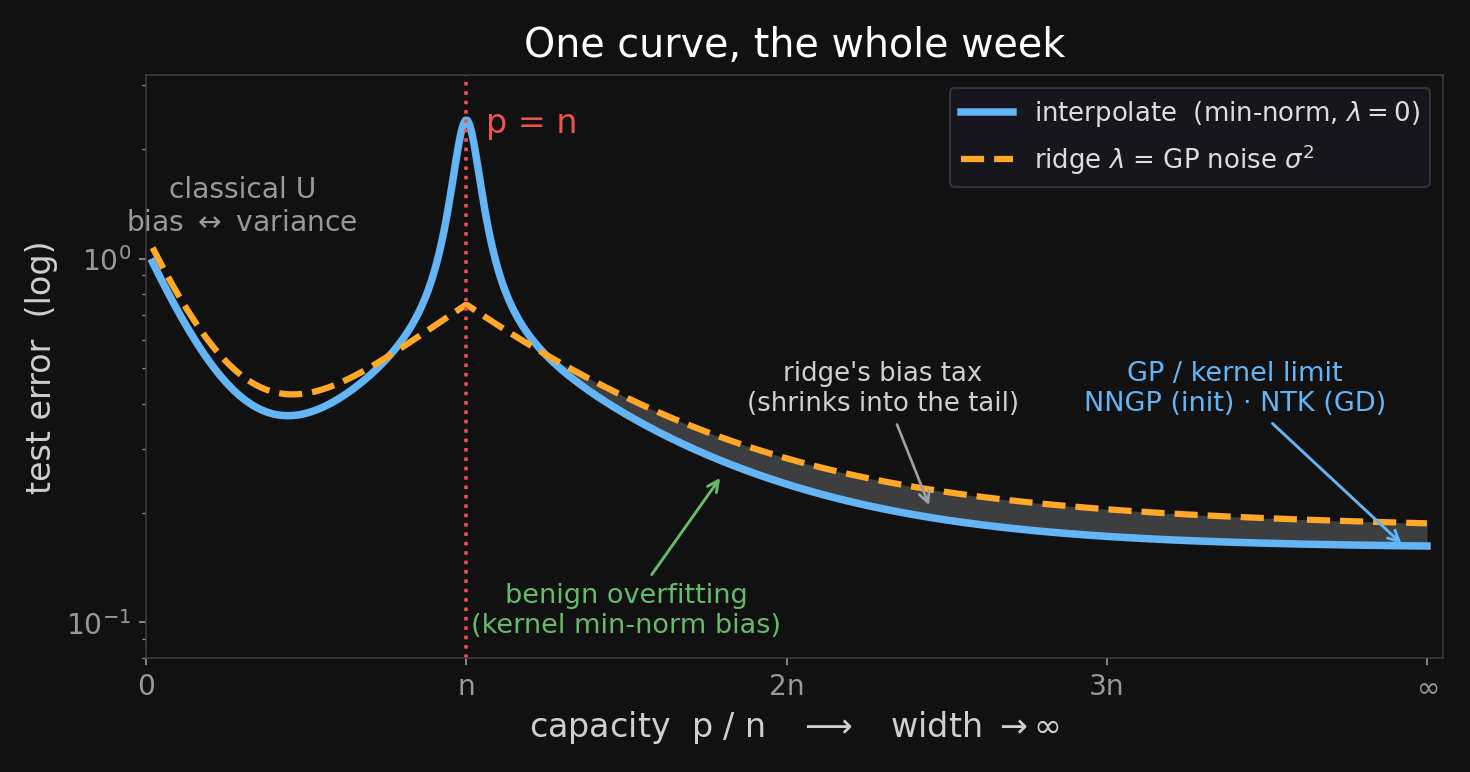
We do not resolve all three here — Gaussian processes are a chapter of their own, and the next chapter takes up the nonparametric road. But you should leave with the picture that regularizing, growing capacity, and pinning a prior over functions are three views of one idea: every model needs a way to prefer some explanations over others, and that preference — the prior — is what controls complexity.

Further Reading

• Geman, Bienenstock, & Doursat (1992), “Neural Networks and the Bias/Variance Dilemma,” Neural Computation 4(1), 1–58 — the paper that named the dilemma and made the U-curve canonical.
• Belkin, Hsu, Ma, & Mandal (2019), “Reconciling modern machine-learning practice and the classical bias-variance trade-off,” PNAS 116(32), 15849–15854 — the double-descent curve, stated as a unifying picture.
• Nakkiran, Kaplun, Bansal, Yang, Barak, & Sutskever (2019), “Deep Double Descent: Where Bigger Models and More Data Hurt” — double descent in real deep networks, including over training time.
• Nakkiran, Venkat, Kakade, & Ma (2020), “Optimal Regularization Can Mitigate Double Descent” — optimally tuned ridge removes the double-descent peak; the formal version of Section 7’s “ridge, honestly.”
• Bartlett, Long, Lugosi, & Tsybakov (2020), “Benign overfitting in linear regression,” PNAS 117(48), 30063–30070 — why interpolation can generalize, and the high-dimensional conditions it requires.
• Hastie, Montanari, Rosset, & Tibshirani (2019/2022), “Surprises in High-Dimensional Ridgeless Least Squares Interpolation,” Annals of Statistics — the precise high-dimensional asymptotics behind the minimum-norm interpolant.

This material was developed for the “Narrative Introduction to Probability” textbook, generously funded by the [Japanese Probabilistic Computing Consortium Association (JPCCA)](https://jpcca.org/).