Discrete Bayesian Nonparametrics
The Problem with Fixed K
In Chapter 5, we solved Chibany’s bento mystery using a Gaussian Mixture Model (GMM) with K=2 components. But we had to specify K in advance and use BIC to validate our choice.
What if:
- We don’t know how many types exist?
- The number of types changes over time?
- We want the model to discover the number of clusters automatically?
The honest difficulty is that “how should we cluster these points?” has an astronomical number of answers. The number of ways to partition $n$ points into groups is the Bell number $B_n$, and it explodes far faster than the $2^n$ subsets of a set — by $n = 15$ there are already over a billion possible clusterings.
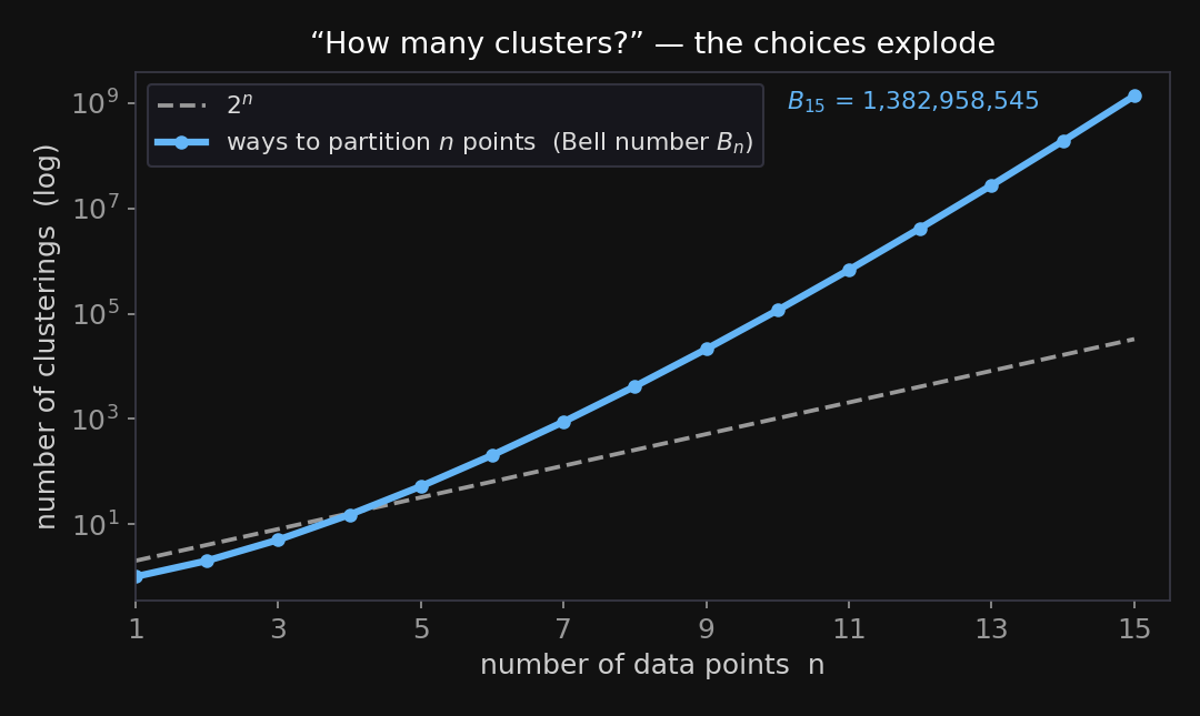
We cannot enumerate clusterings; we need a prior over partitions that a sampler can explore. Bayesian nonparametrics supplies one. The word “nonparametric” is a misnomer — these models have infinitely many parameters, not zero. The point is that the effective number of parameters (here, clusters) is not fixed in advance; it grows with the data.
Enter the Dirichlet Process Mixture Model (DPMM): a Bayesian nonparametric model that learns the number of components from the data. This chapter is about the object underneath it — the Dirichlet Process (DP) — and the family of “let the data choose the cardinality” models it unlocks.
One Object, Three Lenses
Almost everything written about the DPMM introduces three constructions — the Chinese Restaurant Process, the Pólya urn, and stick-breaking — and it is easy to come away thinking they are three different models. They are not. They are three lenses on one object: the Dirichlet Process. Getting this straight now will save you real confusion later.
The object: a random distribution
A draw $G \sim \mathrm{DP}(\alpha, G_0)$ is not a number and not a vector — it is a random probability distribution. It has two knobs:
- the base measure $G_0$ — where the atoms of $G$ tend to land (for our bentos, $G_0 = \mathcal{N}(\mu_0, \sigma_0^2)$, the prior on a cluster’s mean weight $\mu_k$);
- the concentration $\alpha > 0$ — how the unit of probability splits up among atoms (small $\alpha$ → a few dominant atoms; large $\alpha$ → many small ones).
The single most important fact about the DP is this:
Why a DPMM clusters at all
A draw $G \sim \mathrm{DP}(\alpha, G_0)$ is almost surely discrete — even when the base measure $G_0$ is a smooth, continuous density. All of $G$’s probability piles up on a countable set of atoms $\theta_1, \theta_2, \dots$ with weights $\pi_1, \pi_2, \dots$:
$$G = \sum_{k=1}^{\infty} \pi_k\, \delta_{\theta_k},$$where $\delta_{\theta}$ is a point mass at $\theta$. (In DP notation each atom is written $\theta_k$; for our bentos $\theta_k = \mu_k$, the cluster’s Gaussian mean weight introduced just above.)
Why is a DP draw discrete — what forces all that mass onto a countable comb of spikes? The stick-breaking construction (Lens 3, below) is the mechanism: it breaks the unit stick of probability into a countably infinite set of positive weights $\pi_1, \pi_2, \dots$, and pins each one to its own atom $\theta_k \sim G_0$ — so a draw is literally $G = \sum_{k=1}^{\infty} \pi_k\, \delta_{\theta_k}$, discrete by construction, not by magic. Contrast a plain continuous measure (or a Gaussian process): it smears its mass smoothly, puts zero probability on any single point, and so independent draws from it never repeat a value. The DP is designed to do the opposite — to make repeated draws $\theta \sim G$ land on the same atoms, with positive probability.
Because $G$ is discrete, drawing parameters $\theta \sim G$ independently therefore produces ties — the same atom comes up again and again. A tie is exactly two data points sharing a cluster. The clustering in a DPMM is not bolted on; it falls out of the discreteness of $G$.
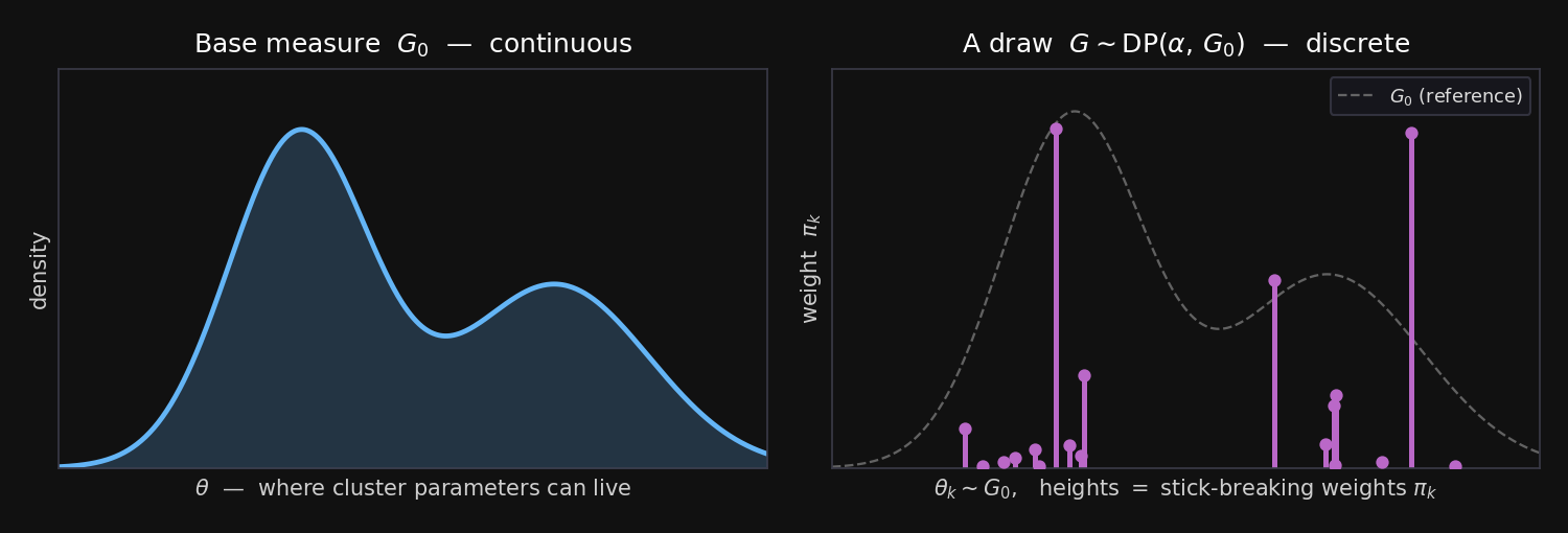
The picture is the whole idea: feed in a continuous $G_0$ (left), and a DP draw hands back a discrete $G$ (right) — a comb of spikes at locations $\theta_k \sim G_0$ with heights $\pi_k$. Now the three “constructions” are just three ways of looking at this comb:
| Lens | What it describes | A.k.a. |
|---|---|---|
| Stick-breaking | builds $G$ explicitly — the spike heights $\pi_k$ and locations $\theta_k$ | Sethuraman (1994); GEM($\alpha$) weights |
| Pólya urn | the DP’s predictive marginal — draw $\theta_1, \theta_2, \dots \sim G$, then integrate $G$ out | Blackwell–MacQueen (1973) |
| Chinese Restaurant Process | the partition those draws induce (who shares with whom) | a Kingman paintbox |
A terminology trap worth getting right
People often say “we put a DP on the assignments” when they really mean the Pólya urn / CRP. Keep the distinction sharp:
- The Dirichlet process is the random measure $G$ itself (the comb of spikes). Stick-breaking constructs it.
- The Pólya urn (Blackwell–MacQueen 1973) is the DP’s predictive marginal — what the sequence of parameter draws looks like after you integrate $G$ out. It is a consequence of the DP, not the DP.
- The Chinese Restaurant Process is the law of the partition those draws induce, forgetting the actual parameter values. By Kingman’s paintbox theorem, every such exchangeable partition arises from sampling labels from a random discrete measure exactly like $G$ — so the CRP partition is a Kingman paintbox painted with the DP’s weights.
In short: one object (the DP), seen as a construction (stick-breaking), as a predictive rule (Pólya urn), or as a partition (CRP).
We now walk the three lenses, starting with the friendliest.
Lens 1 — The Chinese Restaurant Process (the partition)
The most intuitive lens on the DP is the Chinese Restaurant Process (CRP).
The Setup
Imagine a restaurant with infinitely many tables (each table represents a cluster). Customers (observations) enter one by one and choose where to sit:
Rule: Customer n+1 sits:
- At an occupied table k with probability proportional to the number of customers already there: $\frac{n_k}{n + \alpha}$
- At a new table with probability: $\frac{\alpha}{n + \alpha}$
Where:
- nₖ = number of customers at table k
- α = “concentration parameter” (controls tendency to create new tables)
- n = total customers so far
The Rich Get Richer
This creates a rich-get-richer dynamic:
- Popular tables attract more customers (clustering)
- But there’s always a chance of starting a new table (flexibility)
- α controls the trade-off: larger α → more new tables
Connecting to Bentos
- Customer = bento observation
- Table = cluster (bento type)
- Seating choice = cluster assignment
- α = how likely new bento types appear
The dish at a table is a Gaussian center
The restaurant metaphor has one more piece, and it is the bridge to the actual model. Each table serves a dish — a parameter $\theta_k$ drawn once from the menu $G_0$ when the table opens, and shared by everyone seated there. For Chibany’s bentos the menu is $G_0 = \mathcal{N}(\mu_0, \sigma_0^2)$, so the dish is a cluster’s Gaussian mean, $\theta_k = \mu_k \sim G_0$. Opening a new table means drawing a fresh Gaussian center; a customer’s observed weight is then $x_i \sim \mathcal{N}(\theta_{\text{table}(i)}, \sigma_x)$. The CRP decides the partition (who sits together); the dishes $\theta_k$ decide where each cluster sits on the weight axis.
Watch the seating dynamics — and how $\alpha$ tunes the appetite for new tables — in the widget below.
Drive it yourself
Press Auto-seat and watch the rich-get-richer dynamic: the first few tables grab most customers, and the bar at the top shows the probability the next customer opens a brand-new table (∝ $\alpha$). Now drag $\alpha$: near $\alpha = 0.2$ almost everyone crowds onto one or two tables; near $\alpha = 5$ the restaurant sprays customers across many small tables. The number of tables is never fixed — the data grow it. (Static fallback: see the discovered-clusters figure later in the chapter.)
Lens 2 — The Pólya Urn (the DP’s predictive marginal)
The CRP told us who sits with whom but threw away the dish values. Put the dishes back in and you get the Pólya urn of Blackwell & MacQueen (1973) — the same sequential rule, now tracking the actual parameters $\theta_i$:
$$\theta_{n+1} \mid \theta_1, \dots, \theta_n \;\sim\; \frac{\alpha}{n+\alpha}\, G_0 \;+\; \frac{1}{n+\alpha}\sum_{i=1}^{n} \delta_{\theta_i}.$$In words: the next parameter is, with probability $\frac{\alpha}{n+\alpha}$, a brand-new draw from $G_0$ (open a new table, get a new dish), and otherwise a copy of one of the parameters already seen (sit at an existing table, eat its dish) — each existing value reused in proportion to how many times it has already appeared. That reuse is the rich-get-richer dynamic, expressed over parameter values instead of table labels.
Here is the subtle and important part — where does this rule come from? Imagine drawing $\theta_1, \dots, \theta_{n+1} \stackrel{\text{iid}}{\sim} G$ from a single random measure $G \sim \mathrm{DP}(\alpha, G_0)$. Conditional on $G$ the draws are independent, so the joint factors as
$$p(\theta_{1:n+1},\, G) = p(G)\,\prod_{i=1}^{n+1} p(\theta_i \mid G).$$Now marginalize the random measure away — integrate $G$ out of the joint:
$$p(\theta_{1:n+1}) = \int p(G)\,\prod_{i=1}^{n+1} p(\theta_i \mid G)\; dG.$$By the DP’s conjugacy and exchangeability this integral is tractable, and the resulting predictive $p(\theta_{n+1} \mid \theta_{1:n})$ collapses to exactly the rule above: with probability $\propto n_k$, copy an existing atom $\theta^*_k$; with probability $\propto \alpha$, draw a fresh $\theta \sim G_0$. The crucial point is that $G$ no longer appears on the right-hand side — only the past draws and $G_0$ remain. That is why the Pólya urn is the DP’s predictive marginal, not the DP itself: it is the random measure averaged out, what one parameter draw predicts about the next once the underlying random distribution has been integrated away. (Blackwell & MacQueen (1973) — and Pitman’s later work on exchangeable partitions — give the full proof. This same marginalization is what makes “collapsed” Gibbs samplers for the DPMM possible: you never have to represent the infinite $G$.)
Lens 3 — Stick-Breaking (the explicit construction of $G$)
The CRP and Pólya urn are marginal views — they never write down $G$. Stick-breaking (Sethuraman, 1994) is the opposite: it constructs the random measure $G$ directly, giving us the spike heights $\pi_k$ and locations $\theta_k$ from the picture above. Put the contrast in one line: the CRP describes the seating order of customers $1, 2, 3, \dots$ arriving one at a time, while stick-breaking builds the weights $\pi_1, \pi_2, \dots$ of the measure directly — the same DP seen as a process over arrivals versus a construction of the measure. This is the lens our GenJAX code will use.
The Process
Imagine a stick of length 1. We break it into pieces:
For k = 1, 2, 3, …, ∞:
- Sample βₖ ~ Beta(1, α)
- Set πₖ = βₖ × (1 - π₁ - π₂ - … - πₖ₋₁)
In plain English:
- β₁ = fraction of stick we take for component 1
- Remaining stick: 1 - β₁
- β₂ = fraction of remaining stick we take for component 2
- π₂ = β₂ × (1 - π₁)
- And so on…
Result: π₁, π₂, π₃, … sum to 1 (they’re valid mixing proportions), with later components getting exponentially smaller shares.
The Beta Distribution
βₖ ~ Beta(1, α) determines how much of the remaining stick we take:
- α large (e.g., α=10): Breaks are more even → many components with similar weights
- α small (e.g., α=0.5): First few breaks take most of the stick → few dominant components
Heights and locations: this is $G$
Stick-breaking gives the heights $\pi_1, \pi_2, \dots$ of the spikes in the $\mathrm{DP}$ picture. The locations are just as simple: each atom gets an independent draw $\theta_k \sim G_0$ from the base measure (for us, a Gaussian center $\mu_k \sim \mathcal{N}(\mu_0, \sigma_0^2)$). Together they are the random measure:
$$G = \sum_{k=1}^{\infty} \pi_k\, \delta_{\theta_k}, \qquad \pi_k = \beta_k \textstyle\prod_{jThe widget below puts two of our lenses side by side at the same $\alpha$: stick-breaking (top) explicitly breaks a unit stick into the weights $\pi_k$, while the Pólya urn (bottom) draws balls one at a time by the predictive rule. Same object, two mechanisms.
Drive it yourself
Drag $\alpha$ and watch both panels react together. At small $\alpha$ the stick’s first piece $\pi_1$ swallows most of the unit length and the urn fills with mostly one color — a few big clusters. At large $\alpha$ the stick shatters into many thin pieces and the urn shows many colors — many small clusters. The two panels never look identical (different random draws), but they always tell the same story about how many clusters $\alpha$ produces, because they are the same object. (Static fallback: the $G_0 \to G$ figure above shows one such discrete draw.)
The Partition Law (EPPF)
We can now close the loop between the lenses with a single formula. Run the CRP to seat $n$ customers and you get a partition — a grouping of the $n$ points into $K$ blocks of sizes $n_1, \dots, n_K$. What is the probability of that partition? Multiply the CRP’s one-customer-at-a-time probabilities along the arrival order and the product simplifies — the numerators collect each table’s within-table arrival factors $1 \cdot 2 \cdots (n_k - 1)$, while the denominators combine into one running normalizer — and, remarkably, you get the same value for every order consistent with the partition. That common value is the exchangeable partition probability function (EPPF):
$$P(\text{partition}) \;=\; \frac{\alpha^{K}\,\prod_{k=1}^{K}(n_k - 1)!}{\alpha(\alpha+1)\cdots(\alpha+n-1)}.$$Every piece is readable:
- $\alpha^{K}$ — each of the $K$ occupied tables “cost” a factor $\alpha$ to open. More tables ⇒ a higher power of $\alpha$, so larger $\alpha$ favors more clusters. This is the rich-get-started term.
- $\prod_k (n_k-1)!$ — rewards big tables (a table of size $n_k$ contributes $(n_k-1)!$). This is the rich-get-richer term: lopsided partitions (a few large blocks) are far more probable than evenly-split ones.
- $\alpha(\alpha+1)\cdots(\alpha+n-1)$ — the normalizer (the rising factorial $\alpha^{(n)}$). It is the product of the seating rule’s per-customer normalizers: when the $i$-th customer arrives (for $i = 0, 1, \dots, n-1$) she sees $i$ customers already seated plus the new-table mass $\alpha$, a normalizer of $(i + \alpha)$; multiplying these across all $n$ arrivals gives $\prod_{i=0}^{n-1}(i+\alpha) = \alpha(\alpha+1)\cdots(\alpha+n-1)$.
The defining feature is what is absent: the formula depends only on the block sizes $\{n_k\}$, not on which customer is which or the order they arrived. That invariance is exchangeability, and it is what lets a Gibbs sampler pluck any point out and reseat it as if it were the last to arrive.
Connecting back to stick-breaking (at a handwave). Stick-breaking built the discrete $G = \sum_k \pi_k \delta_{\theta_k}$ explicitly. Draw $\theta_1, \dots, \theta_n$ i.i.d. from this $G$: each draw lands on atom $k$ with probability $\pi_k$, and two draws collide — share a cluster — whenever they pick the same atom. If you write down the probability of a given collision pattern and average over the random stick weights $\pi$ (which are GEM($\alpha$)-distributed) and over which atom is which, you recover exactly the EPPF above. So the three lenses are provably one object: stick-breaking’s weights generate the very partition law the CRP and Pólya urn write down directly. (The full calculation is in Pitman’s work on exchangeable partitions; we take the agreement as given.)
DPMM for Gaussian Mixtures: The Full Model
Model Specification
Stick-breaking (infinite components):
- For k = 1, 2, …, K_max:
- βₖ ~ Beta(1, α)
- π₁ = β₁
- πₖ = βₖ × (1 - Σⱼ₌₁ᵏ⁻¹ πⱼ) for k > 1
Component parameters:
- μₖ ~ N(μ₀, σ₀²) [prior on means]
Observations (using stick-breaking weights directly):
- For i = 1, …, N:
- zᵢ ~ Categorical(π) [cluster assignment using stick-breaking weights]
- xᵢ ~ N(μ_zᵢ, σₓ²) [observation from assigned cluster]
Important: We use the stick-breaking weights π directly for cluster assignment. Adding an extra Dirichlet draw would create “double randomization” that makes inference much slower and less accurate!
Why K_max?
In practice, we truncate the infinite model at some large K_max (e.g., 10 or 20). As long as K_max > the true number of clusters, this approximation is accurate.
Implementing DPMM in GenJAX
Let’s implement the DPMM for Chibany’s bentos using the corrected approach:
| |
Output:
Generated data: [-10.4  -9.9 -10.1   0.1   9.9  10.2 ...]
Cluster assignments: [0, 0, 0, 5, 3, 3, 3, ...]
Notice: The model automatically discovered active clusters (0, 3, 5 in this run), ignoring the others!
Inference: A Slice Sampler for the DPMM
Now let’s condition on Chibany’s actual bento weights and infer the clusters. This is harder than the forward direction, and the choice of inference algorithm matters a lot.
Why not plain importance sampling?
The tempting first idea is to sample whole DPMMs from the prior and keep the ones that match the data (importance/rejection sampling). It fails badly here: a random 10-component stick-breaking draw almost never places its means near three tight clusters at $-10, 0, +10$, so essentially every sample gets a vanishingly small weight. We need an algorithm that moves toward the data instead of guessing blindly.
The slice-sampling idea
The classic solution is the slice sampler of Walker (2007). Its trick is to introduce one auxiliary “slice” variable per observation:
$$u_i \sim \text{Uniform}(0,\ \pi_{z_i})$$where $\pi_{z_i}$ is the mixing weight of the cluster $i$ currently belongs to, and $\text{Uniform}(a,b)$ is the uniform distribution on the interval $[a,b]$.
Why is this useful? Given the slice values, a component $k$ is only a candidate for observation $i$ if its weight clears the slice, $\pi_k > u_i$. Because the stick-breaking weights shrink geometrically, only finitely many components ever clear the slice — so even though the model has infinitely many potential clusters, each sweep only has to consider a finite, adaptive set. The number of active clusters $K$ can grow or shrink from sweep to sweep as the data demand, which is exactly the behavior a nonparametric model should have. (We still allocate a generous truncation KMAX as a storage bound, but the slice — not the truncation — decides how many clusters are live.)
The Gibbs sweep
Each sweep cycles through four conditional updates, sampling each quantity given the current value of the others:
- Slice variables $u_i \sim \text{Uniform}(0, \pi_{z_i})$ — set the per-observation thresholds.
- Assignments $z_i$ — pick a cluster from those allowed by the slice, weighted by how well it explains $x_i$: $ P(z_i = k) \propto \mathbb{1}[\pi_k > u_i] \mathcal{N}(x_i \mid \mu_k, \sigma_x)$, where $\mathbb{1}[\cdot]$ is the indicator (1 if true, 0 if false).
- Stick weights $\beta_k \sim \text{Beta}(1 + n_k,\ \alpha + \sum_{j>k} n_j)$, where $n_k$ is the number of observations now in cluster $k$ — the standard stick-breaking posterior.
- Cluster means $\mu_k$ — a conjugate Normal–Normal update from the points assigned to cluster $k$ (empty clusters fall back to the prior).
We keep the explicit for-loops over sweeps so each step is readable; a later chapter shows how to vectorize with scan.
| |
Output:
=== DPMM slice sampler (300 sweeps, 100 burn-in, seed 0) ===
Discovered 3 active clusters
  Cluster 0: mu = -10.03   (n = 5)
  Cluster 1: mu =   0.29   (n = 1)
  Cluster 2: mu =  10.25   (n = 5)

Posterior over number of clusters K:
  P(K = 3) = 0.58
  P(K = 4) = 0.35
  P(K = 5) = 0.07
The sampler recovers all three clusters — the five $\approx -10$ bentos, the lone $\approx 0$ bento, and the five $\approx +10$ bentos — and learns their means accurately. The posterior over $K$ also reflects genuine uncertainty in the number of clusters: $K=3$ is most probable, but the model gives real weight to a spurious fourth or fifth cluster — something a fixed-$K$ GMM cannot express at all.
A caveat: the posterior over $K$ is a treacherous object
It is tempting to read “$P(K = 3) = 0.58$” as the model’s calibrated belief about how many clusters really exist. Be careful — the marginal posterior over the number of clusters is a deep and nuanced object, and for the DPMM it does not behave the way you might hope.
Miller & Harrison (2014) proved that the DPMM’s posterior on the number of clusters is inconsistent: even when the data truly come from a finite mixture with a fixed number of components, as you collect more and more data the marginal posterior over $K$ keeps spawning extra clusters and never settles on the right number. Strikingly, this happens even while the model does density estimation perfectly well — the predictive distribution is fine, the joint is well-estimated; it is specifically the count $K$ that misbehaves. So a DPMM is an excellent density estimator and a treacherous cluster-counter.
The good news is that this is fixable, and the fix is one careful practitioners often reach for anyway. Ascolani, Lijoi, Rebaudo & Zanella (2022) showed that putting a prior on the concentration parameter $\alpha$ — rather than fixing it, as we did with ALPHA = 1.0 above — recovers consistency for the number of clusters when the data are generated from a finite mixture. Letting $\alpha$ itself be learned (the same “hyperprior on the prior” move you’ll see in Chapter 12) is exactly the elegant remedy. The practical upshot: trust the DPMM’s predictive fit and its clustering of the data, but treat any single number for “how many clusters” with suspicion unless you’ve put a prior on $\alpha$.
Slice values do the truncation
We allocated KMAX = 20 storage slots, but never assumed 20 clusters: in any sweep, only the components whose weight clears some observation’s slice ($\pi_k > u_i$) are live. The data, through the slice, decide how many clusters exist — which is the whole point of going nonparametric.
The same sampler on real bento weights
We used abstract weights at $-10, 0, +10$ to keep the three clusters obvious. The Week-10 lecture runs this same slice-sampled DPMM on realistic bento weights in grams: eight Hamburger bentos near 350 g, six Tonkatsu near 500 g — and one stray 275 g bento. With no $K$ specified, the sampler settles on three clusters, and the lone light bento earns its own table rather than being forced into the 350 g group. That is the nonparametric promise made concrete: let the data decide how complex the model should be.
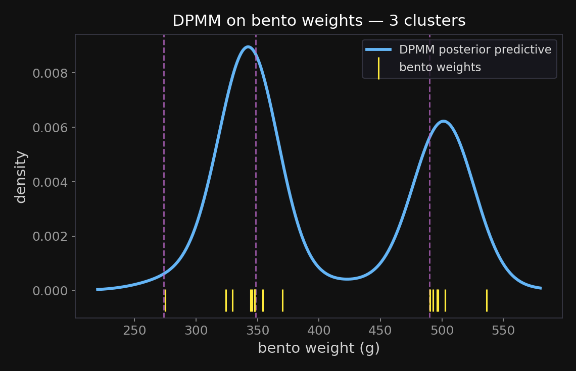
The blue curve is the posterior predictive density — a mixture of the discovered Gaussian clusters — and the dashed lines are the recovered centers $\theta_k$. The 275 g outlier produces a small, low third mode: the model is genuinely uncertain whether it is a rare third type or a fluke, which is precisely the kind of structured uncertainty a fixed-$K$ GMM cannot express. (This figure is generated by the lecture backbone genjax_dpmm.py, which shares the exact Gibbs machinery you just ran above.)
Analyzing the Posterior
The sampler gives us a collection of clusterings (one per post-burn-in sweep), not a single answer. Summarizing them takes a little care because of label switching: the cluster we call “0” in one sweep might be called “2” in the next, since the labels are arbitrary. So we cannot just average mu_0 across sweeps — that average mixes different physical clusters together and is meaningless.
Two summaries that are meaningful:
(1) A single representative clustering — take the final sweep and relabel its clusters left-to-right by their mean, so the numbering is interpretable:
| |
Output:
Cluster assignment per bento: [0, 0, 0, 0, 0, 1, 2, 2, 2, 2, 2]

Cluster means:
  Cluster 0: μ = -10.03   (n = 5)
  Cluster 1: μ =   0.29   (n = 1)
  Cluster 2: μ =  10.25   (n = 5)
(2) A label-invariant summary — the co-clustering probability that two bentos land in the same cluster, averaged over all samples. This sidesteps label switching entirely, because “same cluster?” doesn’t depend on what the cluster is named:
| |
Output:
Co-clustering probability matrix P(i ~ j):
  [1.00 0.92 0.90 0.88 0.90 0.00 0.00 0.00 0.00 0.00 0.00]
  [0.92 1.00 0.88 0.87 0.93 0.00 0.00 0.00 0.00 0.00 0.00]
  [0.90 0.88 1.00 0.88 0.88 0.00 0.00 0.00 0.00 0.00 0.00]
  [0.88 0.87 0.88 1.00 0.90 0.00 0.00 0.00 0.00 0.00 0.00]
  [0.90 0.93 0.88 0.90 1.00 0.00 0.00 0.00 0.00 0.00 0.00]
  [0.00 0.00 0.00 0.00 0.00 1.00 0.00 0.00 0.00 0.00 0.00]
  [0.00 0.00 0.00 0.00 0.00 0.00 1.00 0.90 0.93 0.90 0.86]
  [0.00 0.00 0.00 0.00 0.00 0.00 0.90 1.00 0.88 0.86 0.90]
  [0.00 0.00 0.00 0.00 0.00 0.00 0.93 0.88 1.00 0.88 0.90]
  [0.00 0.00 0.00 0.00 0.00 0.00 0.90 0.86 0.88 1.00 0.86]
  [0.00 0.00 0.00 0.00 0.00 0.00 0.86 0.90 0.90 0.86 1.00]
The block structure is unmistakable: the five $\approx -10$ bentos (rows 0–4) almost always share a cluster with each other and never with the rest; the lone $\approx 0$ bento (row 5) sits by itself; the five $\approx +10$ bentos (rows 6–10) form the third block. The model recovered the three groups without ever being told there were three — and the within-block probabilities sitting a little below 1.0 honestly reflect the small chance, seen in the posterior over $K$, that a group occasionally splits.
A Trap: Label Switching
We sidestepped a subtle but important problem above, and it’s worth making explicit because it bites every mixture model, not just the DPMM.
The cluster labels are arbitrary. Nothing in the model distinguishes “cluster 0” from “cluster 2” — the likelihood
$$p(x \mid z, \mu) = \prod_i \mathcal{N}(x_i \mid \mu_{z_i}, \sigma_x)$$is completely unchanged if we swap the names of two clusters and swap their means to match. The model has a built-in symmetry: with $K$ occupied clusters there are $K!$ equivalent labelings of the same clustering, all with identical posterior probability.
Why this breaks naive summaries. A good sampler will, over many sweeps, wander between these equivalent labelings — the group sitting at $-10$ might be called cluster 0 in one sweep and cluster 2 in the next. So if you compute a per-label average like
$$\bar\mu_0 = \frac{1}{S}\sum_{s} \mu_0^{(s)},$$you are averaging the $-10$ group’s mean in some sweeps with the $+10$ group’s mean in others. The result is mush — typically a number near the overall data mean with a huge standard deviation, which looks like a failed inference even when the sampler worked perfectly. (Try it: averaging mu_0 across our sweeps gives something like $\mu \approx 0 \pm 9$, which is nonsense — the sampler is fine; the summary is wrong.)
The fixes — all of which we used or could use here:
- Report label-invariant quantities. The co-clustering matrix above never asks “what is cluster $k$?”, only “are $i$ and $j$ together?”, so label switching simply cannot affect it. This is the most robust option and the one to reach for first. The posterior over the number of clusters $K$ is label-invariant too.
- Summarize a single representative sample, not an average across samples — e.g. the final sweep (or the highest-posterior sweep), relabeled into a canonical order. That’s what
mode_assignmentsdid: we sorted the clusters left-to-right by mean so “cluster 0” always denotes the lightest group. - Impose an identifiability constraint / relabel post hoc. Pin an ordering (e.g. $\mu_0 < \mu_1 < \mu_2$) or run a relabeling algorithm (Stephens, 2000) that permutes each sweep’s labels to best match a reference before averaging. Then per-label averages become meaningful again.
Don’t average raw per-label parameters
If you find yourself writing jnp.mean(mu_k for each sweep) over MCMC samples of a mixture model, stop. Either summarize a label-invariant function of the clustering, or relabel the samples into a canonical order first. Raw per-label averages silently conflate different clusters and make a healthy sampler look broken.
The Posterior Predictive Distribution
Question: What weight should Chibany expect for the next bento?
To predict the next bento’s weight, we draw from the recovered mixture: pick a cluster in proportion to how many bentos it holds, then sample a weight from that cluster’s Gaussian. We use the representative (final-sweep) clustering for a clean, interpretable predictive.
| |
Output:
Posterior predictive mean: 0.21
Posterior predictive std:  9.72
  P(next bento ≈ -10) = 0.45
  P(next bento ≈  0) = 0.09
  P(next bento ≈ +10) = 0.46
The posterior predictive is multimodal — a mixture of the three clusters — so its overall mean ($\approx 0$) is not a sensible prediction: no bento actually weighs around zero. The useful statement is the per-mode breakdown: the next bento is about equally likely to be a light ($\approx -10$) or heavy ($\approx +10$) type, with a small chance of the rare middle type. Let’s visualize it!
Visualizing the Results
| |
Click to show visualization code
| |
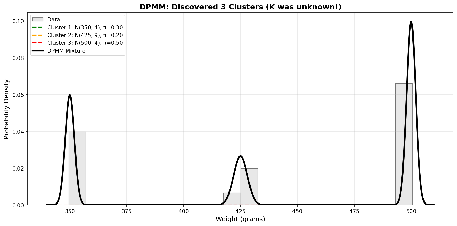
The visualization shows:
- Left: Observed data points with posterior cluster centers and uncertainties
- Right: Trimodal posterior predictive (mixture of three Gaussians)
Comparing DPMM to Fixed-K GMM
| Feature | Fixed-K GMM | DPMM |
|---|---|---|
| K specified? | Yes (must choose K) | No (learned from data) |
| Model selection | BIC, cross-validation | Automatic |
| New clusters | Requires refitting | Discovered automatically |
| Computational cost | Lower (fixed K) | Higher (infinite K, truncated) |
| Uncertainty in K | Not modeled | Naturally captured |
When to use DPMM:
- Unknown number of clusters
- Exploratory data analysis
- Data arrives sequentially (online learning)
- Want Bayesian uncertainty quantification
When to use Fixed-K GMM:
- K is known or strongly constrained
- Computational efficiency matters
- Simpler implementation preferred
See all three density estimators at once
The widget below estimates the density of a set of bento weights three ways simultaneously: a DPMM (lets the data choose the number of clusters), a KDE (kernel density estimate — a bump on every point, no clusters at all), and a fixed-K GMM (you pick $K$). Click on the plot to add a bento weight and watch all three update live.
Drive it yourself
Start with the three clusters preloaded. Drag the GMM $K$ down to 2 and add a few points far to the right — the fixed-$K$ fit cannot grow a new mode and smears one Gaussian to cover them, while the DPMM simply spins up a fourth cluster. Then crank the KDE bandwidth $h$: too small and it spikes on every point; too large and the three modes blur into one. The DPMM needs no such knob — it reads the cluster count off the data via $\alpha$. (Static fallback: the discovered-clusters figure earlier in the chapter.)
The Role of α (Concentration Parameter)
α controls the tendency to create new clusters:
| |
Click to show visualization code
| |
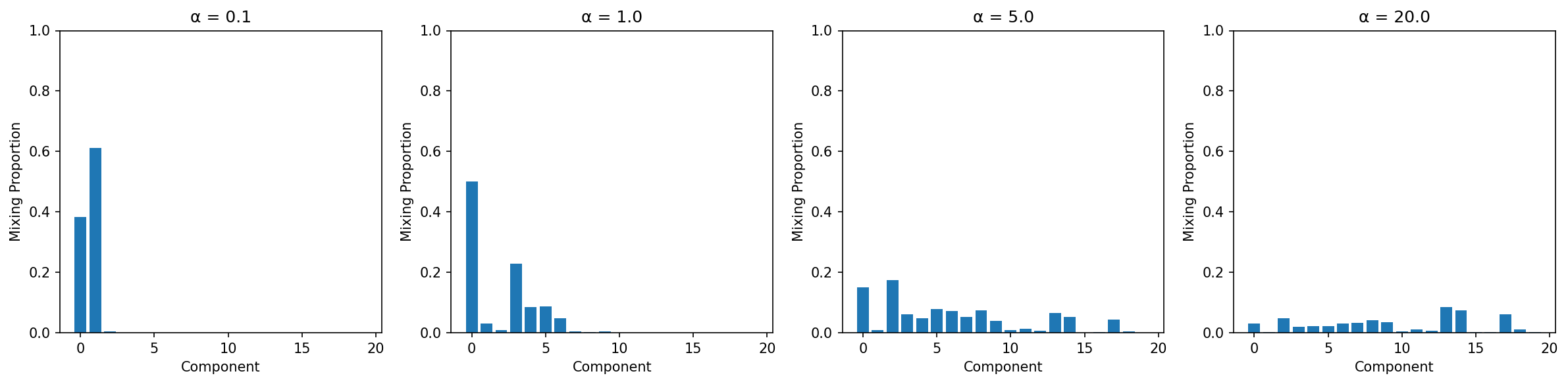
Interpretation:
- α = 0.1: First component dominates (few clusters)
- α = 1.0: Moderate spread (balanced)
- α = 5.0: More components active (many clusters)
- α = 20.0: Very even spread (diffuse)
The DP as a Building Block: One Machine, Many Models
Here is the payoff for all this machinery, and it is bigger than clustering. There is one structural move behind every Bayesian nonparametric model:
Replace a finite parameter with a random measure, and let the data decide how much of it to use.
A finite mixture has a finite parameter — a length-$K$ vector of mixing weights $\pi \sim \mathrm{Dirichlet}(\alpha/K, \dots, \alpha/K)$ over exactly $K$ clusters. Take the limit $K \to \infty$ and that finite Dirichlet vector becomes the random measure $G \sim \mathrm{DP}(\alpha, G_0)$ we have been studying. The DPMM is just “finite Gaussian mixture, with this one substitution.” But the substitution is modular: drop a DP (or a cousin) into any model that has a “how many?” knob, and the knob disappears — the data set it. Three examples show the range.
Topics: from LDA to HDP-LDA
Latent Dirichlet Allocation (LDA; Blei, Ng & Jordan, 2003) is the canonical topic model. Each topic is a distribution over words (“lunch” leans on bento, rice, sauce; “studying” leans on exam, study, grade), and each document is a mixture over a fixed number $T$ of topics, with the per-document topic proportions drawn from a finite Dirichlet. It works beautifully — but you must choose $T$, the very fixed-cardinality problem we started with, one level up.
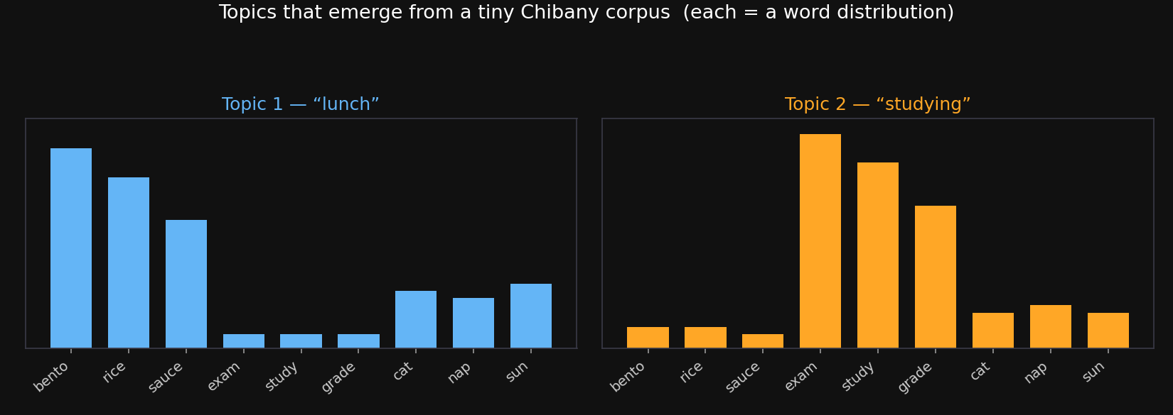
Apply the move. Replace the finite topic Dirichlet with a Dirichlet process and you get HDP-LDA (Teh, Jordan, Beal & Blei, 2006), which learns the number of topics from the corpus. The “H” is Hierarchical, and it is essential: a top-level DP draws a shared global menu of topics, and each document gets its own DP that draws from that shared menu. Without the hierarchy, each document’s DP would invent private topics that never align across documents; the shared base measure is what lets two documents reuse the same topic. The HDP is exactly the “stack a prior on the prior” idea from Chapter 12 (Hierarchical Bayes) — applied to a random measure instead of a scalar.
Features: the Indian Buffet Process
The DP/CRP gives each item exactly one cluster — one table per customer. But many objects are better described by a set of present-or-absent features: a face has glasses and a beard and a hat; a gene belongs to several pathways at once. The feature analogue of the CRP is the Indian Buffet Process (IBP; Griffiths & Ghahramani, 2011). Customers file past an infinitely long buffet and sample each dish (feature) independently, with probability proportional to how many earlier customers took it, plus a $\mathrm{Poisson}(\alpha/n)$ helping of brand-new dishes. Each object walks away with a binary feature vector over an unbounded set of features — not a single label.
The relationship mirrors the DP exactly. Just as the CRP/Pólya urn is the predictive marginal of the Dirichlet process, the IBP is the predictive marginal of the Beta process (Thibaux & Jordan, 2007) — the DP’s sibling, a random measure whose draws are subsets rather than single assignments. Same recipe (“put a prior on a measure of unbounded size”), different measure, and clusters become features.
The honest status of the DPMM in 2026
As a stand-alone clustering algorithm, the DPMM is now somewhat niche. If you only want point clusters, a well-tuned finite mixture or a method like HDBSCAN is often simpler and faster, and — as the Miller–Harrison result above warns — the DPMM’s cluster count needs care (put a prior on $\alpha$). Reviewers rarely reach for a vanilla DPMM to cluster a dataset today.
As a building block, the DP is everywhere. Its real value is as a reusable, modular “unknown-cardinality” prior you drop inside a larger model: topic models (HDP), feature models (IBP / Beta process), infinite HMMs, nonparametric mixtures of experts, and Bayesian components of neural models. The reason to learn the Dirichlet process is less “a clustering tool” and more “a Lego brick for models that grow with the data.” Master the three lenses, and you can read — and build — that whole family.
Real-World Applications
Anomaly Detection
- Normal data forms clusters
- Outliers create singleton clusters
- α controls sensitivity to outliers
Topic Modeling
- Documents are mixtures over topics
- DPMM discovers number of topics automatically
- Each topic is a distribution over words
Genomics
- Cluster genes by expression patterns
- Number of functional groups unknown
- DPMM identifies distinct expression profiles
Image Segmentation
- Pixels cluster by color/texture
- DPMM finds natural segments
- No need to specify number of segments
Practice Problems
Problem 1: Adjusting α
Using the observed bento data from earlier, run inference with α ∈ {0.5, 2.0, 10.0}.
a) How does the number of active clusters change?
b) How does posterior uncertainty change?
Show Solution
We reuse the gibbs_sweep from earlier, just rerunning the sampler at each $\alpha$ and reporting the average number of occupied clusters (averaging over sweeps, which avoids the single-sweep noise):
| |
Output:
α =  0.5:  E[K] = 3.21
α =  2.0:  E[K] = 3.60
α = 10.0:  E[K] = 4.76
The trend is exactly as the theory predicts: a larger concentration parameter $\alpha$ makes the model spin up more clusters (some of them spurious splits of the three real groups), while a small $\alpha$ keeps it parsimonious. Note that even at $\alpha = 0.5$ the model still finds the three genuine clusters — the data are clearly separated enough that the likelihood overrides the prior’s pull toward fewer clusters.
Problem 2: Sequential Learning
Chibany receives bentos one at a time. Implement online learning where the model updates as each bento arrives.
Hint: One simple approach reuses the slice sampler you already have — after each new bento arrives, rerun the sampler on all data seen so far and report the occupied clusters. (A more efficient approach would warm-start from the previous posterior instead of restarting; that is the idea behind sequential Monte Carlo.)
Show Solution (sketch)
This is left as an implementation exercise. The structure below is pseudo-code — run_sampler is the function from Problem 1; the point is the outer loop over a growing data prefix, not a new inference algorithm:
| |
Expected behavior: the number of occupied clusters grows as genuinely new bento types first appear, then stabilizes once each type has been seen — the model commits to a new cluster only when the data force it to.
What We’ve Accomplished
We started with a mystery: bentos with an average weight that doesn’t match any individual bento. Through this tutorial, we:
- Chapter 1: Understood expected value paradoxes in mixtures
- Chapter 2: Learned continuous probability (PDFs, CDFs)
- Chapter 3: Mastered the Gaussian distribution
- Chapter 4: Performed Bayesian learning for parameters
- Chapter 5: Built Gaussian Mixture Models with Bayesian posterior inference
- Chapter 6: Extended to infinite mixtures with the Dirichlet Process — one object seen through three lenses (CRP, Pólya urn, stick-breaking), and a building block far beyond clustering
You now have the tools to:
- Model complex, multimodal data
- Discover latent structure automatically
- Quantify uncertainty in clustering
- Perform Bayesian inference with GenJAX
Where this goes next
Clustering was about finding structure in a pile of data. The chapters ahead turn the same Bayesian machinery toward new questions:
- Chapter 7: Bayesian Generalization asks how you learn a concept from a handful of examples — the same posterior-over-hypotheses idea, but now the hypotheses are sets (rules), and the payoff is a model of how humans generalize.
- Chapters 8–11: the Bayesian-networks spine zoom out from a single model to the structure of models: drawing them as graphs (Bayes nets), reading off which variables inform which (conditional independence and d-separation), distinguishing seeing from doing (causal Bayes nets and the do-operator), and measuring it all in bits (information theory). The DPMM you just built is itself a Bayes net — Chapter 8 makes that explicit.
- Chapter 12: Hierarchical Bayes stacks priors on priors so the model can learn its own prior from related problems — and, as we noted above, it’s exactly the move that tames the DPMM’s cluster-count behavior.
So the mystery bentos were just the beginning: the rest of Tutorial 3 is about graphs, causes, information, and learning the prior itself.
Further Reading
Theoretical Foundations (the three lenses)
- Ferguson (1973): “A Bayesian Analysis of Some Nonparametric Problems” (defines the DP)
- Blackwell & MacQueen (1973): “Ferguson Distributions via Pólya Urn Schemes” (the Pólya urn — the DP’s predictive marginal)
- Sethuraman (1994): “A Constructive Definition of Dirichlet Priors” (the stick-breaking construction)
- Kingman (1978): “The Representation of Partition Structures” (the paintbox theorem behind the CRP)
- Pitman (1995): “Exchangeable and Partially Exchangeable Random Partitions” (the EPPF / partition law)
- Austerweil, Gershman, Tenenbaum, & Griffiths (2015): “Structure and Flexibility in Bayesian Models of Cognition” (Chapter in The Oxford Handbook of Computational and Mathematical Psychology - comprehensive overview of Bayesian nonparametric approaches to cognitive modeling)
The DP as a building block
- Blei, Ng & Jordan (2003): “Latent Dirichlet Allocation” (the finite-$T$ topic model)
- Teh, Jordan, Beal & Blei (2006): “Hierarchical Dirichlet Processes” (HDP-LDA — the nonparametric topic model)
- Griffiths & Ghahramani (2011): “The Indian Buffet Process: An Introduction and Review” (nonparametric features)
- Thibaux & Jordan (2007): “Hierarchical Beta Processes and the Indian Buffet Process” (the Beta process — the IBP’s underlying random measure)
Practical Implementations
- Neal (2000): “Markov Chain Sampling Methods for Dirichlet Process Mixture Models” (MCMC inference)
- Walker (2007): “Sampling the Dirichlet Mixture Model with Slices” (the slice sampler used in this chapter)
- Kalli, Griffin, & Walker (2011): “Slice sampling mixture models” (refinements and a clear exposition)
- Blei & Jordan (2006): “Variational Inference for Dirichlet Process Mixtures” (scalable inference)
- Stephens (2000): “Dealing with label switching in mixture models” (post-hoc relabeling for valid per-component summaries)
GenJAX Documentation
- GenJAX GitHub - Official repository
- Probabilistic Programming Examples - Gen.jl (sister project)
Key Takeaways
- One object, three lenses: the Dirichlet Process $G \sim \mathrm{DP}(\alpha, G_0)$ is one random discrete distribution. Stick-breaking (Sethuraman) constructs it; the Pólya urn (Blackwell–MacQueen) is its predictive marginal (integrate $G$ out); the CRP is the partition it induces (a Kingman paintbox). They are not three models.
- Why a DPMM clusters: a DP draw is almost surely discrete, so i.i.d. parameter draws $\theta \sim G$ repeat — and a repeat is two points sharing a cluster. The dish $\theta_k \sim G_0$ is a cluster’s Gaussian mean.
- EPPF: the partition probability $\dfrac{\alpha^{K}\prod_k (n_k-1)!}{\alpha(\alpha+1)\cdots(\alpha+n-1)}$ depends only on block sizes — that invariance is exchangeability. Larger α ⇒ more clusters.
- Slice sampler: auxiliary slice variables $u_i$ adaptively truncate the infinite stick, so each Gibbs sweep handles only finitely many live clusters.
- Label switching: cluster labels are arbitrary — summarize with label-invariant quantities (co-clustering, posterior over $K$) or a single relabeled sample, never raw per-label averages.
- A building block, not just a clustering tool: the move “finite parameter → random measure” recurs everywhere — HDP topic models (the nonparametric LDA) and the IBP / Beta process for features. The DPMM-as-clustering is niche; the DP as a Lego brick is everywhere.
Glossary: Dirichlet Process · concentration $\alpha$ · base measure · Chinese Restaurant Process · Pólya urn · stick-breaking · EPPF · Kingman paintbox · HDP · LDA · IBP · Beta process
Interactive Exploration
Want to experiment with DPMMs yourself? Try our interactive Jupyter notebook that lets you:
- Adjust the concentration parameter α and see its effect on clustering
- Add or remove data points and watch the model adapt
- Change the truncation level K_max
- Visualize posterior distributions in real-time
Try It Yourself!
📓 Open Interactive DPMM Notebook on Google Colab
No installation required - runs directly in your browser!
The notebook includes:
- Complete DPMM implementation with stick-breaking
- Interactive widgets for all parameters
- Real-time visualization of posteriors
- Guided exercises to deepen understanding
This is a great way to build intuition for how α, K_max, and the data itself interact to produce the posterior distribution.
References
- Antoniak, C. E. (1974). Mixtures of Dirichlet processes with applications to Bayesian nonparametric problems. The Annals of Statistics, 2(6), 1152–1174. https://doi.org/10.1214/aos/1176342871
- Ascolani, F., Lijoi, A., Rebaudo, G., & Zanella, G. (2023). Clustering consistency with Dirichlet process mixtures. Biometrika, 110(2), 551–558. https://doi.org/10.1093/biomet/asac051
- Austerweil, J. L., Gershman, S. J., Tenenbaum, J. B., & Griffiths, T. L. (2015). Structure and flexibility in Bayesian models of cognition. In J. R. Busemeyer, Z. Wang, J. T. Townsend, & A. Eidels (Eds.), The Oxford handbook of computational and mathematical psychology (pp. 187–208). Oxford University Press.
- Blackwell, D., & MacQueen, J. B. (1973). Ferguson distributions via Pólya urn schemes. The Annals of Statistics, 1(2), 353–355. https://doi.org/10.1214/aos/1176342372
- Blei, D. M., & Jordan, M. I. (2006). Variational inference for Dirichlet process mixtures. Bayesian Analysis, 1(1), 121–143. https://doi.org/10.1214/06-BA104
- Blei, D. M., Ng, A. Y., & Jordan, M. I. (2003). Latent Dirichlet allocation. Journal of Machine Learning Research, 3, 993–1022. https://www.jmlr.org/papers/v3/blei03a.html
- Ferguson, T. S. (1973). A Bayesian analysis of some nonparametric problems. The Annals of Statistics, 1(2), 209–230. https://doi.org/10.1214/aos/1176342360
- Griffiths, T. L., & Ghahramani, Z. (2011). The Indian buffet process: An introduction and review. Journal of Machine Learning Research, 12, 1185–1224. https://www.jmlr.org/papers/v12/griffiths11a.html
- Kalli, M., Griffin, J. E., & Walker, S. G. (2011). Slice sampling mixture models. Statistics and Computing, 21(1), 93–105. https://doi.org/10.1007/s11222-009-9150-y
- Kingman, J. F. C. (1978). The representation of partition structures. Journal of the London Mathematical Society, s2-18(2), 374–380. https://doi.org/10.1112/jlms/s2-18.2.374
- Miller, J. W., & Harrison, M. T. (2014). Inconsistency of Pitman–Yor process mixtures for the number of components. Journal of Machine Learning Research, 15(96), 3333–3370. https://jmlr.org/papers/v15/miller14a.html
- Neal, R. M. (2000). Markov chain sampling methods for Dirichlet process mixture models. Journal of Computational and Graphical Statistics, 9(2), 249–265. https://doi.org/10.1080/10618600.2000.10474879
- Pitman, J. (1995). Exchangeable and partially exchangeable random partitions. Probability Theory and Related Fields, 102(2), 145–158. https://doi.org/10.1007/BF01213386
- Sethuraman, J. (1994). A constructive definition of Dirichlet priors. Statistica Sinica, 4(2), 639–650. https://www.jstor.org/stable/24305538
- Stephens, M. (2000). Dealing with label switching in mixture models. Journal of the Royal Statistical Society: Series B (Statistical Methodology), 62(4), 795–809. https://doi.org/10.1111/1467-9868.00265
- Teh, Y. W., Jordan, M. I., Beal, M. J., & Blei, D. M. (2006). Hierarchical Dirichlet processes. Journal of the American Statistical Association, 101(476), 1566–1581. https://doi.org/10.1198/016214506000000302
- Thibaux, R., & Jordan, M. I. (2007). Hierarchical beta processes and the Indian buffet process. In Proceedings of the 11th International Conference on Artificial Intelligence and Statistics (AISTATS) (PMLR 2, pp. 564–571). https://proceedings.mlr.press/v2/thibaux07a.html
- Walker, S. G. (2007). Sampling the Dirichlet mixture model with slices. Communications in Statistics — Simulation and Computation, 36(1), 45–54. https://doi.org/10.1080/03610910601096262