Continuous Bayesian Nonparametrics: Gaussian Processes

From Partitions to Functions

The Dirichlet Process Mixture Model of the last chapter answered the question “how many clusters are there?” without ever fixing the number. It did this by putting a prior over an infinite object — a partition of the data into groups — and letting the data decide how many groups light up. That is the whole spirit of Bayesian nonparametrics (BNP): don’t fix the size of the model; put a prior over an infinite-dimensional space and let the posterior keep only as much structure as the data support.

The DPMM’s infinite object was discrete: a partition is a way of chopping the data into a countable set of clusters. This chapter takes up the continuous member of the same family. Instead of a prior over partitions, we place a prior directly over functions — smooth curves $f : \mathbb{R} \to \mathbb{R}$ — and condition on noisy observations to get a posterior over functions. That object is a Gaussian process (GP), and it is the continuous twin of everything you just learned.

What you already have, and what is new

This chapter assumes Chapter 5 (Gaussian mixtures), Chapter 6 (the DPMM — a prior over partitions), and especially Chapter 5a, The Bias-Variance Dilemma. From 5a you should carry three things: the “how complex should the model be?” question, ridge regression (a Gaussian prior on coefficients that shrinks the fit), and the boxed identity it ended on — $\lambda = \sigma^2$, the ridge penalty equals the observation-noise variance. That identity was advertised there as “the bridge to Gaussian processes.” This chapter walks across that bridge and, at the end, resolves the trilogy 5a opened.

Brand new here, and defined as we go: kernels and the length-scale, the Gaussian process prior and posterior, the marginal likelihood as a kernel-chooser, and the deep link to neural networks — NNGP and the NTK — plus their modern echoes (neural processes, and retrieval as memory: RAG / kNN-LM).

You should be comfortable with Gaussians, posteriors, $\mathbb{E}[\cdot]$, and basic GenJAX (@gen, simulate, normal). The rest is built here.

Kernels: The Shape of “Nearby”

A prior over functions sounds abstract — a function has infinitely many values, one at every input $x$. The trick that makes it concrete is to never write down a whole function at once. Instead we describe how any two function values co-vary: if $x$ and $x'$ are close, then $f(x)$ and $f(x')$ should be close too. A kernel $k(x, x')$ is exactly that — a function that scores how similar two inputs are, and therefore how tightly their outputs are tied together.

This similarity structure is encoded as a covariance matrix. When the prior is Gaussian and the observation noise is Gaussian, the posterior is also Gaussian — giving closed-form inference, no MCMC needed.

The workhorse kernel is the RBF (radial basis function), also called the squared-exponential kernel:

It has two knobs, and each is a familiar idea wearing a new hat:

• $\sigma_f$ — the signal standard deviation: how far the function swings up and down (the prior marginal std of $f(x)$ is $\sigma_f$).
• $\ell$ — the length-scale: how far a point’s influence reaches. Two inputs closer than $\ell$ are strongly correlated; far past $\ell$ they are nearly independent.

Let’s read the RBF kernel as a similarity that decays with distance. With $\sigma_f = 1$ and $\ell = 0.15$:

 1
 2
 3
 4
 5
 6
 7
 8
 9
10
11
12
13
14

import jax
import jax.numpy as jnp

def rbf_kernel(xa, xb, sig_f=1.0, ell=0.15):
    """RBF (squared-exponential) Gram matrix:
       k(x, x') = sig_f**2 * exp(-(x - x')**2 / (2 * ell**2))."""
    d = xa[:, None] - xb[None, :]
    return (sig_f ** 2) * jnp.exp(-(d ** 2) / (2.0 * ell ** 2))

# How similar are two points a distance r apart? (sig_f = 1, ell = 0.15)
ref = jnp.array([0.0])
for r in [0.0, 0.05, 0.15, 0.30, 0.60]:
    k = float(rbf_kernel(ref, jnp.array([r]))[0, 0])
    print(f"  distance r = {r:.2f}   ->   k = {k:.4f}")

Output:

  distance r = 0.00   ->   k = 1.0000
  distance r = 0.05   ->   k = 0.9460
  distance r = 0.15   ->   k = 0.6065
  distance r = 0.30   ->   k = 0.1353
  distance r = 0.60   ->   k = 0.0003

At zero distance the similarity is maximal ($\sigma_f^2 = 1$). At exactly one length-scale ($r = \ell = 0.15$) it has dropped to $e^{-1/2} \approx 0.607$, and by four length-scales ($r = 0.60$) two points are effectively unrelated. The kernel is the inductive bias: choosing $\ell$ is choosing how wiggly you believe the truth is, before you have seen a single data point. Small $\ell$ → the kernel is spiky → function values even a little apart become nearly independent → the model expects rapid wiggling. Large $\ell$ → the kernel decays slowly → distant points stay correlated → the model expects smooth, slow change. Hold onto that — it is the thread the whole chapter pulls.

The GP Prior and Posterior

Here is the definition that makes all of this computable. A Gaussian process is a prior over functions such that any finite set of function values is jointly Gaussian. Pick any inputs $x_1, \dots, x_n$; then the vector $\big(f(x_1), \dots, f(x_n)\big)$ is a draw from a multivariate normal with mean $\mathbf{m}$ (we use zero) and covariance matrix $K_{ij} = k(x_i, x_j)$ built from the kernel. That’s it — the kernel is the covariance. We never represent the whole infinite function; we only ever ask for its values on a finite grid, and those are Gaussian.

Sampling prior functions with the Cholesky trick (GenJAX)

We can’t sample the infinite-dimensional GP directly, so we discretize to the $n$ grid points; there the joint prior is $\mathcal{N}(\mathbf{0}, K)$. The Cholesky factor $L$ is a linear transform that turns white noise $\mathbf{z}\sim\mathcal{N}(\mathbf{0},I)$ into correlated samples $\mathbf{f} = L\mathbf{z}$ with exactly $LL^\top = K$.

How do you draw a whole function from this prior? On a grid of $n$ points we need a sample from $\mathcal{N}(\mathbf{0}, K)$. The Cholesky trick does it with nothing but independent standard normals: factor $K = L L^\top$ (with $L$ lower-triangular), draw $\mathbf{z} \sim \mathcal{N}(\mathbf{0}, I)$ — $n$ independent draws — and set $\mathbf{f} = \mathbf{m} + L\mathbf{z}$. Then $\mathbf{f}$ has covariance $L\,\mathbb{E}[\mathbf{z}\mathbf{z}^\top]L^\top = L L^\top = K$, exactly the GP. The correlations are manufactured by $L$ from white noise.

This is a one-liner to write as a GenJAX generative model: the only random choices are the iid latents $z_i \sim \mathcal{N}(0,1)$, and the function is a deterministic linear push-through.

 1
 2
 3
 4
 5
 6
 7
 8
 9
10
11
12
13
14
15
16
17
18
19
20
21
22
23
24
25
26
27
28
29
30
31
32
33
34
35
36
37

from genjax import gen, normal

SIG_F = 1.0      # signal std: prior marginal std of f(x)
ELL   = 0.15     # length-scale: how far a point's influence reaches
JITTER = 1e-6    # tiny diagonal added before Cholesky for stability

def make_gp_prior_model(n_grid):
    """Factory: a GenJAX GP-prior model over a grid of n_grid points.
    n_grid is captured as a Python constant (a closure), NOT a model arg
    (a `for i in range(n)` over a traced arg raises TracerIntegerConversionError).
    The model draws n_grid iid standard normals z and returns f = mu + L @ z."""
    @gen
    def gp_prior(mu, L):
        zs = [normal(0.0, 1.0) @ f"z_{i}" for i in range(n_grid)]
        z = jnp.stack(zs)
        return mu + L @ z          # correlate the latents -> a GP draw
    return gp_prior

def sample_prior_functions(key, grid, sig_f=SIG_F, ell=ELL, n_samples=5):
    n = grid.shape[0]
    K = rbf_kernel(grid, grid, sig_f, ell) + JITTER * jnp.eye(n)
    L = jnp.linalg.cholesky(K)
    mu = jnp.zeros(n)
    model = make_gp_prior_model(n)
    keys = jax.random.split(key, n_samples)
    fs = jax.vmap(lambda k: model.simulate(k, (mu, L)).get_retval())(keys)
    return fs, K, L

grid = jnp.linspace(0.0, 1.0, 120)
key = jax.random.key(0)
k_prior = jax.random.split(key, 3)[1]
prior_samples, K, L = sample_prior_functions(k_prior, grid, n_samples=5)

print(f"  drew {prior_samples.shape[0]} prior functions x {prior_samples.shape[1]} grid points")
# The Cholesky trick is exact: L @ L^T must reconstruct the kernel matrix K.
recon_err = float(jnp.max(jnp.abs(L @ L.T - K)))
print(f"  Cholesky reconstruction  max|L Lᵀ - K| = {recon_err:.2e}")

Output:

  drew 5 prior functions x 120 grid points
  Cholesky reconstruction  max|L Lᵀ - K| = 2.98e-07

Each of those five rows is a complete function — 120 correlated values — sampled from the prior before any data. They are all different (the prior is uncertain about the truth) but all smooth at the scale $\ell$ (the kernel’s doing). The reconstruction check confirms the trick is exact: $L L^\top$ rebuilds $K$ to floating-point precision.

Conditioning on data: the closed-form posterior

Now the payoff of Gaussianity. Because the prior is jointly Gaussian and the observation noise is Gaussian, the posterior is available in closed form — no MCMC. Given training inputs $X$ with noisy targets $y = f(X) + \varepsilon$, $\varepsilon \sim \mathcal{N}(0, \sigma_n^2)$, the posterior over the function at any test inputs $X_\*$ is Gaussian with

Read the mean formula slowly: the prediction at $X_\*$ is a similarity-weighted combination of the observed $y$’s — points near $X_\*$ (high kernel value) get more vote. (Hold that thought; it returns at the very end as retrieval.) We solve the linear systems with a Cholesky factorization for numerical stability.

 1
 2
 3
 4
 5
 6
 7
 8
 9
10
11
12
13
14
15
16
17
18
19
20
21
22
23
24
25
26
27
28
29
30
31
32
33
34
35
36
37
38
39
40
41
42
43
44
45
46
47

import jax.numpy as jnp
from jax.scipy.linalg import cho_factor, cho_solve

SIGMA_N = 0.1    # observation-noise std

def true_function(x):
    """A smooth 1-D test function on [0, 1]."""
    return jnp.sin(2.5 * jnp.pi * x) * jnp.exp(-x)

def make_training_data(key, n=6, noise=SIGMA_N):
    k_x, k_eps = jax.random.split(key)
    base = jnp.linspace(0.05, 0.95, n)
    X = jnp.clip(base + 0.02 * jax.random.normal(k_x, (n,)), 0.0, 1.0)
    y = true_function(X) + noise * jax.random.normal(k_eps, (n,))
    return X, y

def gp_posterior(X, y, Xstar, sig_f=SIG_F, ell=ELL, noise=SIGMA_N):
    """Closed-form GP posterior at Xstar given (X, y):
        K     = k(X,X) + noise**2 I
        mean* = k(X*,X) K^{-1} y
        cov*  = k(X*,X*) - k(X*,X) K^{-1} k(X,X*)."""
    # sig_f / ell default to the module constants SIG_F / ELL set above and are
    # passed explicitly into every rbf_kernel call below, so the kernel here uses
    # the same hyperparameters as the prior sampler unless a caller overrides them.
    n = X.shape[0]
    Kxx = rbf_kernel(X, X, sig_f, ell) + (noise ** 2) * jnp.eye(n)
    Ksx = rbf_kernel(Xstar, X, sig_f, ell)
    Kss = rbf_kernel(Xstar, Xstar, sig_f, ell)
    c = cho_factor(Kxx)
    mean = Ksx @ cho_solve(c, y)
    cov  = Kss - Ksx @ cho_solve(c, Ksx.T)
    std  = jnp.sqrt(jnp.clip(jnp.diag(cov), 0.0, None))
    return mean, cov, std

k_data = jax.random.split(key, 3)[0]
X, y = make_training_data(k_data, n=6)
post_mean, post_cov, post_std = gp_posterior(X, y, grid)

# Sanity: with Gaussian noise the GP SMOOTHS, so the mean at the training
# inputs should match y up to about the noise level (not exactly).
mean_at_train, _, _ = gp_posterior(X, y, X)
print("  posterior mean at training inputs vs observed y:")
print(f"    {'x':>7} {'y (obs)':>9} {'post mean':>10} {'|diff|':>8}")
for xi, yi, mi in zip(X, y, mean_at_train):
    print(f"    {float(xi):7.3f} {float(yi):9.3f} {float(mi):10.3f} {float(abs(mi-yi)):8.4f}")
print(f"  max |post_mean - y| at train pts = {float(jnp.max(jnp.abs(mean_at_train - y))):.4f}"
      f"   (noise std = {SIGMA_N})")

Output:

  posterior mean at training inputs vs observed y:
          x   y (obs)  post mean   |diff|
      0.039     0.161      0.164   0.0028
      0.246     0.691      0.679   0.0127
      0.405    -0.137     -0.129   0.0085
      0.619    -0.445     -0.447   0.0015
      0.760    -0.232     -0.225   0.0070
      0.915     0.349      0.342   0.0073
  max |post_mean - y| at train pts = 0.0127   (noise std = 0.1)

The posterior mean passes within the noise level of every observation — it does not interpolate exactly (that would be overfitting the noise), it smooths, exactly as the $\sigma_n^2$ on the diagonal asks it to. The picture below is the one to keep in your head.

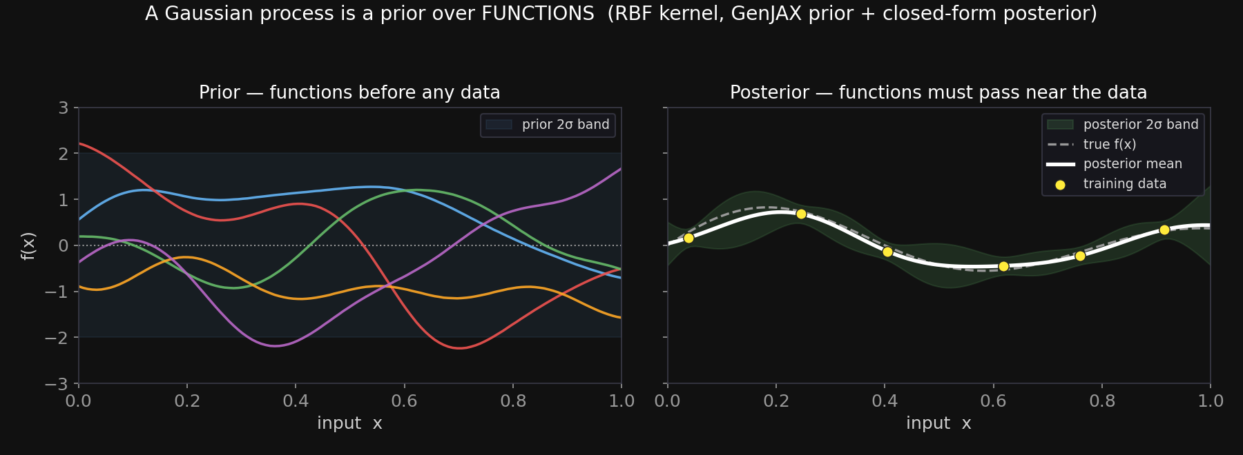
The right panel shows the signature behavior of a GP posterior: the uncertainty band pinches at the data (where observations nail the function down) and widens away from it (where the prior, not the data, is doing the talking). At a training input the posterior-covariance term $k(X_\*, X)\,K^{-1}\,k(X, X_\*)$ subtracts off almost all the prior variance; far from any data that term shrinks and the prior variance dominates — so the band is tight at the data and widens away from it. A GP does not just give you a best-fit curve; it tells you where it is guessing.

 1
 2
 3
 4
 5
 6
 7
 8
 9
10
11
12
13
14
15
16
17
18
19
20
21
22
23
24
25

# Plotting only. This reproduces the two-panel figure above; the published
# version uses the course's dark theme (see course/week10_*/genjax_gp.py).
import matplotlib.pyplot as plt

fig, (axp, axo) = plt.subplots(1, 2, figsize=(12, 4.4), sharey=True)

# Left: prior samples + 2-sigma band
axp.fill_between(grid, -2 * SIG_F, 2 * SIG_F, alpha=0.12, label="prior 2σ band")
for f in prior_samples:
    axp.plot(grid, f, lw=1.5, alpha=0.9)
axp.set_title("Prior — functions before any data")
axp.set_xlabel("input x"); axp.set_ylabel("f(x)"); axp.legend()

# Right: posterior mean + 2-sigma band + data
axo.fill_between(grid, post_mean - 2 * post_std, post_mean + 2 * post_std,
                 alpha=0.2, label="posterior 2σ band")
axo.plot(grid, true_function(grid), ls="--", label="true f(x)")
axo.plot(grid, post_mean, lw=2.5, label="posterior mean")
axo.scatter(X, y, zorder=6, s=55, label="training data")
axo.set_title("Posterior — functions must pass near the data")
axo.set_xlabel("input x"); axo.legend()

plt.tight_layout()
plt.savefig("genjax_gp.png", dpi=150)
plt.show()

Choosing the Kernel: the Marginal Likelihood

We picked $\ell = 0.15$ by hand. But the whole BNP promise is let the data decide — so how does a GP choose its own inductive bias? Through the marginal likelihood (also called the evidence): the probability the model assigns to the observed $y$, with the function itself integrated out. For a GP it, too, is closed form:

The two data-dependent terms pull against each other and automatically encode Occam’s razor: the $y^\top K^{-1} y$ term rewards fitting the data, while the $\log|K|$ term penalizes a kernel flexible enough to fit anything. A more flexible kernel spans a larger prior volume of functions, so it spreads its prior mass thinner — lower prior density on any particular dataset, hence lower evidence. That is Occam’s razor, automatic. Sweep the length-scale and the evidence picks a winner:

 1
 2
 3
 4
 5
 6
 7
 8
 9
10
11
12
13
14
15
16
17
18
19
20
21

import jax.numpy as jnp
from jax.scipy.linalg import cho_factor, cho_solve

def log_marginal_likelihood(X, y, sig_f=SIG_F, ell=ELL, noise=SIGMA_N):
    """GP log marginal likelihood:
       log p(y|X) = -1/2 yᵀ K⁻¹ y  - 1/2 log|K|  - n/2 log 2π,
       with K = k(X,X) + noise² I."""
    n = X.shape[0]
    Kn = rbf_kernel(X, X, sig_f, ell) + (noise ** 2) * jnp.eye(n)
    c = cho_factor(Kn)
    alpha = cho_solve(c, y)
    logdet = 2.0 * jnp.sum(jnp.log(jnp.diag(c[0])))   # log|K| = 2 Σ log diag(L)
    return -0.5 * y @ alpha - 0.5 * logdet - 0.5 * n * jnp.log(2.0 * jnp.pi)

print("  length-scale ℓ   log marginal likelihood")
ells = jnp.array([0.03, 0.08, 0.15, 0.30, 0.60, 1.00])
lmls = jnp.array([log_marginal_likelihood(X, y, ell=float(e)) for e in ells])
for e, lm in zip(ells, lmls):
    star = "   <- best" if lm == jnp.max(lmls) else ""
    print(f"    {float(e):6.2f}        {float(lm):8.3f}{star}")
print(f"  data-preferred length-scale: ℓ = {float(ells[jnp.argmax(lmls)]):.2f}")

Output:

  length-scale ℓ   log marginal likelihood
      0.03          -5.987
      0.08          -5.947
      0.15          -5.223   <- best
      0.30          -5.528
      0.60         -20.881
      1.00         -31.183
  data-preferred length-scale: ℓ = 0.15

The evidence is maximized at $\ell = 0.15$ — which is the scale the data were actually generated at. Too small ($\ell = 0.03$) and the model wastes flexibility explaining noise; too large ($\ell = 0.60$) and it cannot bend fast enough to fit the data, and the evidence collapses. The data chose the kernel. This is the same “let the data decide the model’s complexity” move as the DPMM’s posterior over the number of clusters — here, decided over the smoothness of functions. Maximizing this evidence over $\ell$, $\sigma_f$, and $\sigma_n$ is exactly how GPs are fit in practice.

From Gaussian Processes to Neural Networks

So far a GP looks like a classical statistics tool. Here is the twist that makes it central to modern machine learning: infinitely wide neural networks are Gaussian processes. Three results, in order, and it is worth being precise about what is random, what the limit is, and what each one describes.

Neal (1996): a wide one-layer Bayesian net is a GP

Take a neural network with one hidden layer of width $H$, random weights, and output $f(x) = \frac{1}{\sqrt{H}}\sum_{j=1}^{H} v_j\,\phi(w_j x + b_j)$. With the weights drawn from a prior, $f(x)$ is a sum of $H$ iid random terms. By the Central Limit Theorem, as $H \to \infty$ that sum becomes Gaussian — and jointly Gaussian across any set of inputs. That is the definition of a GP. Its kernel is the expected product of features, $k(x, x') = \mathbb{E}_{w}\!\left[\phi(w\cdot x)\,\phi(w\cdot x')\right]$ — the average, over the weight prior, of how aligned the hidden units are at the two inputs. A wide one-hidden-layer Bayesian neural network, before training, is a draw from a GP.

A neural net’s output is a weighted sum of many nonlinear features; with enough independent features the Central Limit Theorem makes that sum Gaussian — and the covariance between two inputs IS a kernel.

We can watch the CLT happen. Fix two inputs, draw thousands of random nets at several widths, and measure the covariance of their outputs — it should settle onto a fixed value (one entry of the limiting kernel):

 1
 2
 3
 4
 5
 6
 7
 8
 9
10
11
12
13
14
15
16
17
18
19
20
21
22
23
24

import jax
import jax.numpy as jnp

def net_cov(key, xa, xb, H, n_nets=2000):
    """Sample covariance of a 1-hidden-layer random net's output at xa, xb.
       f(x) = (1/sqrt(H)) sum_j v_j tanh(w_j x + b_j),  w,b,v ~ N(0,1)."""
    kw, kb, kv = jax.random.split(key, 3)
    w = jax.random.normal(kw, (n_nets, H))
    b = jax.random.normal(kb, (n_nets, H))
    v = jax.random.normal(kv, (n_nets, H))
    fa = jnp.sum(v * jnp.tanh(w * xa + b), axis=1) / jnp.sqrt(H)
    fb = jnp.sum(v * jnp.tanh(w * xb + b), axis=1) / jnp.sqrt(H)
    cov = jnp.mean((fa - fa.mean()) * (fb - fb.mean()))
    return float(cov), float(jnp.var(fa))

xa, xb = 0.3, 0.9
kk = jax.random.key(1)
print(f"  inputs xa = {xa}, xb = {xb};  as width H grows, the net's")
print(f"  output covariance settles onto a fixed kernel value:")
print(f"    {'width H':>8} {'Cov[f(xa),f(xb)]':>18} {'Var[f(xa)]':>12}")
for H in [10, 100, 1000, 10000]:
    kk, k = jax.random.split(kk)
    cov, var = net_cov(k, xa, xb, H)
    print(f"    {H:8d} {cov:18.4f} {var:12.4f}")

Output:

  inputs xa = 0.3, xb = 0.9;  as width H grows, the net's
  output covariance settles onto a fixed kernel value:
     width H   Cov[f(xa),f(xb)]   Var[f(xa)]
          10             0.3850       0.3945
         100             0.4054       0.4141
        1000             0.3954       0.3975
       10000             0.3937       0.4003

The covariance stops wandering and locks onto $\approx 0.40$ as the width grows: that limiting number is the GP kernel $k(0.3, 0.9)$ for this architecture. The network has become a Gaussian process in front of us.

NNGP (Lee et al., 2018): the same is true for deep nets, at initialization

Neal’s argument is one layer deep. Lee et al. (2018) showed it composes: a deep fully-connected net, with iid random weights, also converges to a GP as every layer’s width goes to infinity. The kernel is built by a layer recursion — the covariance after layer $\ell$ is a fixed deterministic function of the covariance after layer $\ell-1$, applied $L$ times. This limiting kernel is the NNGP kernel (Neural Network Gaussian Process). The consequence is striking: exact Bayesian inference in an infinitely wide deep net equals GP regression with the NNGP kernel — the same closed-form posterior you coded above, no gradient descent anywhere. Crucially, this describes the network’s prior — the distribution over functions the architecture encodes before training.

NTK (Jacot et al., 2018): a wide net trained by gradient descent is also a kernel method

The NNGP is the net at initialization. What about training? Jacot et al. (2018) answered it. Track how the network’s function changes as gradient descent updates the weights. To first order, that change is governed by the Neural Tangent Kernel (NTK), $\Theta(x, x') = \big\langle \nabla_\theta f(x),\, \nabla_\theta f(x') \big\rangle$ — the similarity of the gradients at two inputs. Their result: in the infinite-width limit the NTK is deterministic and constant throughout training. The weights barely move (the “lazy” regime), the network behaves like a linear model in a fixed feature space, and gradient-descent training reduces to kernel regression with the NTK. (“Lazy” means the weights barely move during training — the wide net stays near its random initialization — because feature learning hasn’t kicked in.) This describes the network during training, under gradient descent.

The clean split — and the one big caveat

So: NNGP is the Bayesian prior at initialization; NTK is what gradient descent does. Two faces of “a wide net is a kernel machine.”

The Modern Echoes

The GP idea — predict at a new point by a kernel-weighted vote over data you remember — keeps reappearing in contemporary ML, usually without the name.

• Neural processes (Garnelo et al., 2018). A GP gives calibrated uncertainty but costs an $n \times n$ matrix inversion and a hand-chosen kernel. Neural processes are neural networks trained to imitate a GP: they map a context set of observations to a predictive distribution over functions in a single forward pass, learning the kernel-like inductive bias from many related tasks instead of fixing it. They trade the GP’s exactness for amortized speed and a learned prior — meta-learning wearing a GP’s clothes.

• Nonparametric memory: RAG and kNN-LM. A standard (“parametric”) language model bakes everything it knows into fixed weights. A nonparametric-memory model instead keeps an explicit, growable datastore and looks things up at inference time — the continuous-BNP spirit (let the model grow with the data) applied to LLMs. kNN-LM (Khandelwal et al., 2020) interpolates the model’s next-token distribution with a nearest-neighbor search over a datastore of (context-embedding → next-token) pairs. RAG (Lewis et al., 2020) retrieves relevant documents and conditions generation on them. Look back at the GP posterior mean, $k(X_\*, X)\,K^{-1} y$ — a similarity-weighted combination of remembered outputs. That is exactly what kNN-LM and RAG do, with a learned embedding as the kernel and the corpus as the training set. Retrieval is nonparametric prediction at LLM scale.

It All Comes Home

We can now close the trilogy that the bias-variance chapter opened. It ended on a boxed promise — $\lambda = \sigma^2$ — and three roads out of the “how complex?” question. This chapter is where they meet.

The kernel ridge is the GP noise: $\lambda = \sigma^2$

In 5a, ridge regression added a penalty $\lambda$ that shrank the fit and traded variance for bias. The GP posterior mean is kernel ridge regression, $\text{mean}(X_\*) = k(X_\*, X)\,[K + \lambda I]^{-1} y$, and the ridge knob is literally the GP’s observation-noise variance, $\lambda = \sigma_n^2$. Not an analogy — the same number. Let’s confirm it on our data:

 1
 2
 3
 4
 5
 6
 7
 8
 9
10
11
12
13

import jax.numpy as jnp

# Kernel ridge regression: mean(x*) = k(x*, X) (K + lambda I)^{-1} y.
# Set lambda = sigma_n^2 and it is EXACTLY the GP posterior mean.
lam = SIGMA_N ** 2
Kxx = rbf_kernel(X, X)
Ksx = rbf_kernel(grid, X)
ridge_mean = Ksx @ jnp.linalg.solve(Kxx + lam * jnp.eye(X.shape[0]), y)

gap = float(jnp.max(jnp.abs(ridge_mean - post_mean)))
print(f"  lambda = sigma_n^2 = {lam:.4f}")
print(f"  max | kernel-ridge mean  -  GP posterior mean |  =  {gap:.2e}")
print("  => the ridge knob lambda IS the GP observation-noise variance sigma^2.")

Output:

  lambda = sigma_n^2 = 0.0100
  max | kernel-ridge mean  -  GP posterior mean |  =  2.98e-07
  => the ridge knob lambda IS the GP observation-noise variance sigma^2.

To floating-point precision, the regularization dial from 5a and the noise variance from this chapter are one object. Regularizing is just being Bayesian about noise.

One question, three answers — and they are one object

Recall 5a’s three roads out of “how complex should the model be?”:

1. Regularize — keep a flexible model, shrink it with a prior. That is ridge ($\lambda = \sigma^2$).
2. Grow capacity with the data — never fix complexity; add structure only when the data demand it. That is Bayesian nonparametrics, the DPMM’s prior over partitions.
3. Put a prior over functions — skip coefficients entirely, place a distribution on the space of curves. That is the Gaussian process of this chapter.

They are not three tricks; they are three views of one object, and this chapter is the hinge that fastens them together:

• Road 1 = Road 3: the GP is kernel ridge with $\lambda = \sigma^2$ (just proved).
• Road 2 = Road 3: the GP is the continuous Bayesian nonparametric — a prior over functions instead of partitions — and it picks its own inductive bias (the kernel) by maximizing the marginal likelihood, the very “let the data decide” engine the DPMM used to pick its number of clusters.
• And the bridge back to 5a’s double descent: via NNGP/NTK, an infinitely wide network is a GP. So the floor that the over-parameterized second descent settles onto — the limit of “more capacity” — is the kernel limit, a GP. The benign overfitting that made interpolation safe in high dimensions is the minimum-norm bias of the kernel: among all functions through the data, the GP/kernel solution prefers the smallest-norm one, and that preference is a prior. Capacity taken to infinity does not escape having a prior — it becomes one.

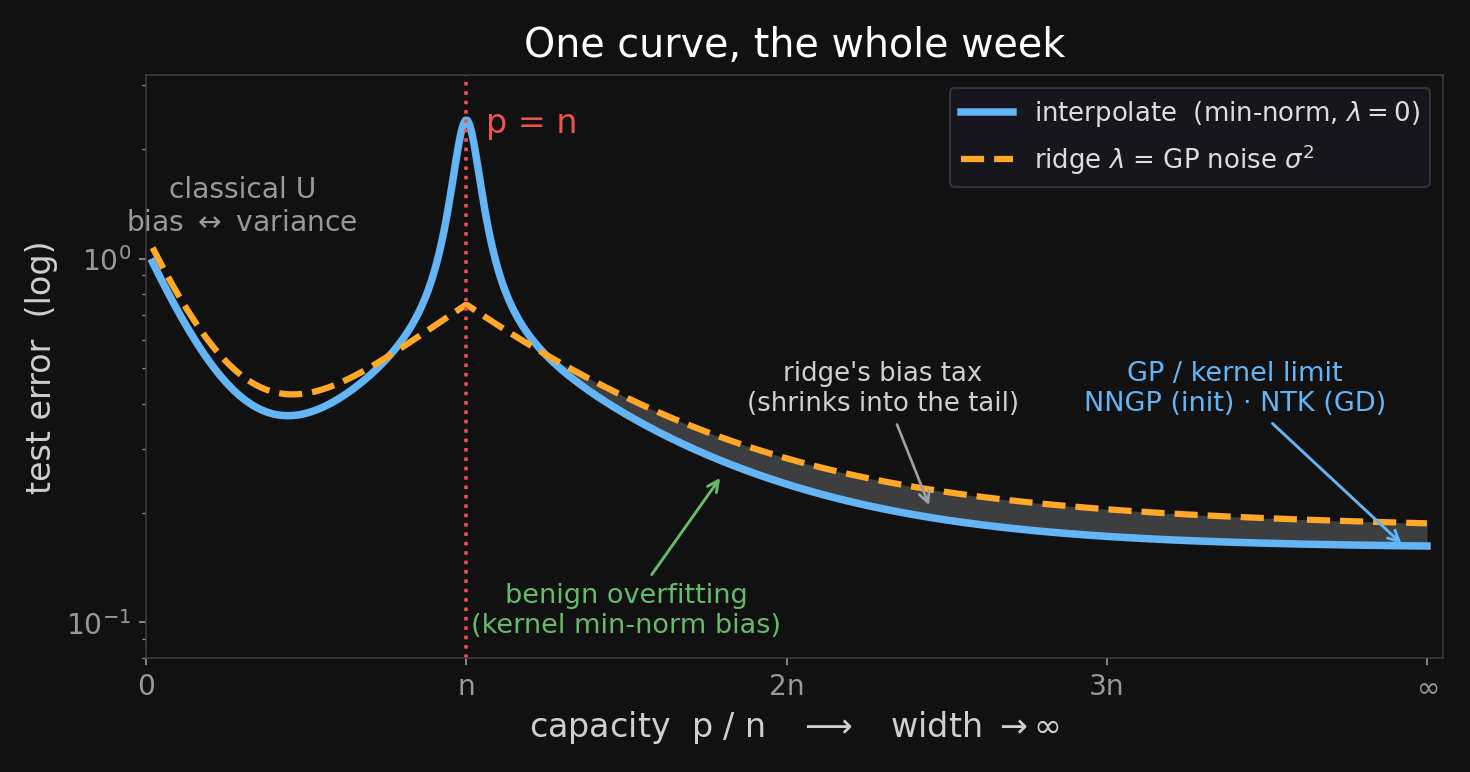
That figure was the cliffhanger at the end of 5a. Now every label on it has a mechanism. The classical U on the left is the bias-variance trade-off. The orange ridge curve that smooths the spike is $\lambda = \sigma^2$. The benign-overfitting tail is the kernel’s minimum-norm prior. And the rightmost limit, where capacity runs to infinity, is the Gaussian-process / kernel limit — the object this whole chapter built. Regularize, grow capacity, prior over functions: one idea, seen from three sides. Every model needs a way to prefer some explanations over others, and that preference — the prior — is what controls complexity.

The next chapter, Bayesian Generalization, keeps the thread: it asks how a learner generalizes a concept from a few examples — the same posterior-over-hypotheses machinery, now where the hypotheses are sets and the payoff is a model of human inductive inference.

Further Reading

• Rasmussen & Williams (2006), Gaussian Processes for Machine Learning, MIT Press — the standard reference; Chapters 2 (regression) and 5 (marginal likelihood / model selection) cover everything in the first half of this chapter, freely available online.
• Neal (1996), Bayesian Learning for Neural Networks, Springer LNS 118 — the thesis that proved a wide one-layer Bayesian net converges to a GP.
• Williams (1997), “Computing with Infinite Networks,” NeurIPS — closed-form kernels for infinitely-wide nets, making Neal’s limit concrete.
• Lee, Bahri, Novak, Schoenholz, Pennington, & Sohl-Dickstein (2018), “Deep Neural Networks as Gaussian Processes,” ICLR — the deep NNGP kernel and the layer recursion.
• Jacot, Gabriel, & Hongler (2018), “Neural Tangent Kernel: Convergence and Generalization in Neural Networks,” NeurIPS — the NTK and the lazy-training picture of gradient descent.
• Chizat, Oyallon, & Bach (2019), “On Lazy Training in Differentiable Programming,” NeurIPS — why the kernel limits lack feature learning.
• Yang & Hu (2021), “Feature Learning in Infinite-Width Neural Networks” (Tensor Programs IV) — the parameterization (µP) under which infinite-width nets do learn features.
• Garnelo, Rosenbaum, Maddison, Ramalho, Saxton, Shanahan, Teh, Rezende, & Eslami (2018), “Conditional Neural Processes,” ICML — neural networks trained to behave like GPs.
• Khandelwal, Levy, Jurafsky, Zettlemoyer, & Lewis (2020), “Generalization through Memorization: Nearest Neighbor Language Models,” ICLR — kNN-LM, nonparametric memory for language.
• Lewis et al. (2020), “Retrieval-Augmented Generation for Knowledge-Intensive NLP Tasks,” NeurIPS — RAG.

This material was developed for the “Narrative Introduction to Probability” textbook, generously funded by the [Japanese Probabilistic Computing Consortium Association (JPCCA)](https://jpcca.org/).