Statistical Decision Theory: From Beliefs to Actions

From Beliefs to Actions

For nineteen chapters we have asked one question, over and over, in a dozen disguises: given what I have seen, what should I believe? We built priors, turned data into likelihoods, and read off posteriors — the whole machinery of Bayesian learning. But a belief is not yet a choice. At some point Chibany has to put down the calculator and eat the bento.

Jamal: “Okay, you’ve computed that the bento is probably fresh. Probably. So — do you eat it?”

Chibany: “Ninety percent fresh. I think… yes?”

Alyssa: “But think about what you’re trading. If it’s fine, you get lunch. If it’s not, you get food poisoning. ‘Probably fresh’ doesn’t tell you what to do — you need to weigh what each mistake costs.”

Alyssa has named the gap this chapter closes. A posterior is a distribution over the world; an action is a single committed move. The bridge between them is statistical decision theory — the normative account of how to turn a belief into a decision once you know what your mistakes cost. It is the hinge of the whole course: everything before today answered what should I believe?; today, the question becomes what should I do?

This chapter is the one-shot version — a single decision, made once. The next chapters stretch it across time, where one action leads to the next and the costs compound.

The Decision Problem

Every decision problem has the same four pieces. We name each one, and its symbol, as we go.

• The state of the world $\theta$ — the thing you don’t know (is the bento fresh or stale?). This is exactly the unknown you have been putting posteriors on all along.
• An observation $x$ — the data you get to see before acting (a sniff, a sell-by date); Weeks 1–7 turned $x$ into a posterior $p(\theta \mid x)$. We keep $x$ a single observation to hold the notation steady, but nothing below changes if it’s a whole batch — you’d simply condition on all of it, $p(\theta \mid x_1, \dots, x_n)$.
• An action $a$, drawn from a set of available actions $A$ (eat, or compost).
• A loss $L(\theta, a)$ — how much you regret taking action $a$ when the world was really $\theta$. Low loss is good (loss is the mirror image of reward, which we’ll meet in the next chapter).

A decision rule $d(x)$ is a strategy: it maps each possible observation to the action you’ll take. The flow runs left to right — the world is hidden, you see a clue, your rule picks an action, and the world’s true state decides what that action cost:

graph LR
    T["hidden state θ"] -.clue.-> X["observation x"]
    X --> D["decision rule d(x)"]
    D --> A["action a"]
    T --> L["loss L(θ, a)"]
    A --> L
    classDef node fill:none,stroke:#9bbcff,stroke-width:2px,color:#fff
    class T,X,D,A,L node
    linkStyle default stroke:#9bbcff,stroke-width:2px,color:#fff

Make the bento concrete. The world is $\theta \in \{\text{fresh}, \text{stale}\}$; the actions are $\{\text{eat}, \text{compost}\}$. The losses say what each combination costs:

Eating a fresh bento is perfect ($0$); eating a stale one is a disaster ($10$); composting wastes a little either way. The numbers encode a value judgment — poisoning is much worse than waste — and decision theory takes that judgment as input. It will not tell you what to care about; it tells you what to do once you have said what you care about.

The table fixes the consequences; the observation is what turns a one-off guess into a rule. Say the one clue Chibany gets is how many days ago the bento was bought, $x$ — a single number. A decision rule $d(x)$ is then any policy from that number to an action, and the natural one is a threshold at some cutoff $k$:

The cutoff $k$ is the rule: a cautious $k = 1$ composts good bentos to play safe (paying the $3$ often), a reckless $k = 6$ eats stale ones (risking the $10$). Which $k$ is right? The more days pass, the likelier the bento has turned — so the answer hinges on a days $\to$ P(fresh) conversion, which we’ll make precise and let GenJAX solve in the In GenJAX section below. First we need a way to score a rule, which is exactly risk.

Risk: the Loss You Expect

You never know $\theta$ when you act, so you can’t minimize $L(\theta, a)$ directly — it depends on the very thing that’s hidden. What you can do is minimize the loss you expect. The risk of a decision rule is its average loss,

the expected loss as the data $x$ varies, for a fixed true state $\theta$. (This $\mathbb{E}$ is the expected value from Chapter 1 and Chapter 16 — a probability-weighted average.) Risk is a report card on a rule: how badly does $d$ do, on average, when the world is $\theta$?

But $\theta$ is itself unknown, so a single rule has a whole curve of risks — one value of $R$ for every possible $\theta$. (If $\theta$ is continuous — say the bento’s weight rather than fresh-or-stale — that curve is literal; for the binary bento it’s just two points, one for fresh and one for stale.) That leaves us a genuine question with two famous answers: how do you collapse a curve of risks into one number to minimize?

Two Ways to Be Optimal: Bayes vs Minimax

The first answer uses your belief. If you think some states of the world are likelier than others, weight the loss by that belief and minimize the average. The Bayes rule minimizes prior-expected risk,

and once you have actually seen your clue $x$, this is equivalent to the move you’ll make for the rest of the course: pick the action that minimizes posterior-expected loss,

Read the subscript: we’ve now fixed $x$ (we took our sniff), so the only uncertainty left is over $\theta$, and we average the loss against the posterior $p(\theta \mid x)$ — not over $x$ as the risk formula did. You have a posterior; you average the loss against it; you take the cheapest action. (That the rule-level $\arg\min_d$ and this action-level $\arg\min_a$ agree is a small theorem; for our purposes the action version is all you ever need.)

The second answer refuses to trust a belief at all. The minimax rule minimizes the worst case — it picks the rule whose highest-possible risk is as low as possible:

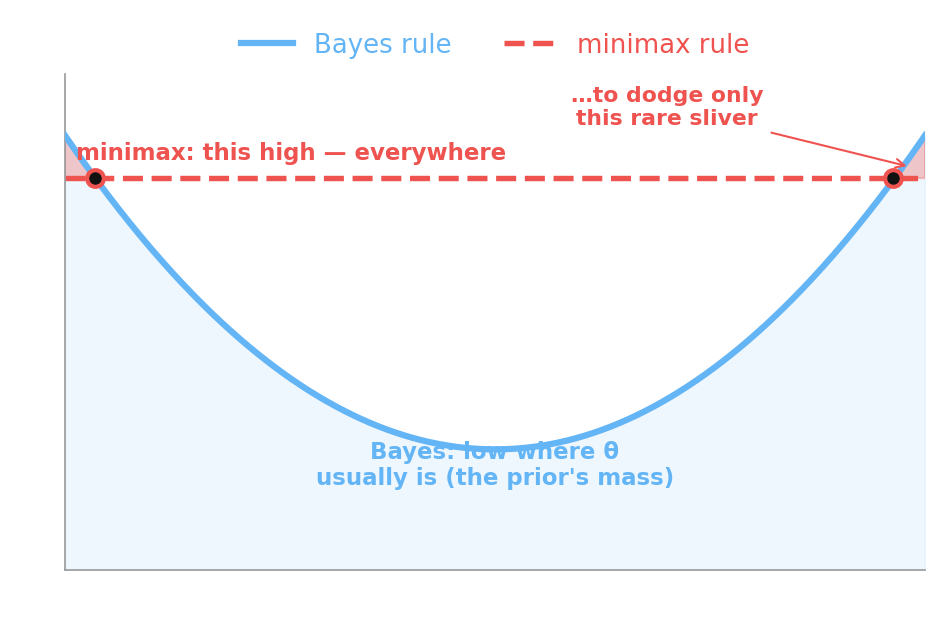
Minimax is the pessimist’s criterion: assume the world is adversarial and protect against the worst it can do. (It is built to flatten its risk across $\theta$ — an “equalizer” rule — which is why it shows up as a flat line in the figure below.) The two criteria can genuinely disagree.

Our first worked example deliberately strips the day-count away — Chibany must commit to a single bento with no observation at all — so a decision rule $d$ collapses to a single action $a$, and risk collapses to the loss itself, $R(\theta, a) = L(\theta, a)$. Bayes then averages that loss over the belief ($\mathbb{E}_\theta$); minimax takes its worst value over $\theta$ (the worst entry down each action’s column). Watch them split on the bento, with a belief that says it’s probably fresh:

1
2
3
4
5
6
7
8
9

import jax
import jax.numpy as jnp
import jax.random as jr

# states theta in {fresh(0), stale(1)}; actions {eat(0), compost(1)}
L = jnp.array([[0.0, 3.0],      # theta = fresh:  eat -> 0,   compost -> 3
               [10.0, 1.0]])     # theta = stale:  eat -> 10,  compost -> 1
belief = jnp.array([0.9, 0.1])   # belief over theta: P(fresh) = 0.9, P(stale) = 0.1
acts = ["eat", "compost"]

1
2
3
4
5
6

exp_loss   = belief @ L                 # belief-weighted (expected) loss: sum over theta of P(theta)*L[theta, a]
worst_case = jnp.max(L, axis=0)         # max over theta (axis 0 = the rows): one worst case per action

print("             eat   compost")
print(f"E[L]       {float(exp_loss[0]):5.2f} {float(exp_loss[1]):5.2f}   ->  Bayes picks {acts[int(jnp.argmin(exp_loss))]}")
print(f"max L      {float(worst_case[0]):5.2f} {float(worst_case[1]):5.2f}   ->  minimax picks {acts[int(jnp.argmin(worst_case))]}")

Output:

             eat   compost
E[L]        1.00  2.80   ->  Bayes picks eat
max L      10.00  3.00   ->  minimax picks compost

The Bayes rule eats: weighing the small $10\%$ chance of poisoning against the usual outcome, the expected loss of eating ($1.00$) beats composting ($2.80$). The minimax rule compostes: it ignores the $90\%$ and stares only at the worst column — eating risks a $10$, composting caps out at $3$, so it refuses to gamble. Neither is “wrong.” They optimize different things: Bayes bets on the prior and wins on average; minimax buys insurance against the catastrophe and pays for it in the typical case.

The picture below is the rule-level view of that trade. The Bayes rule’s risk dips low exactly where the prior says $\theta$ usually lives, at the cost of a thin sliver where it does worse than the flat minimax rule — and that sliver is all the protection minimax buys, everywhere, in exchange for being worse where it counts:

What Loss Are You Minimizing?

Here is the most useful fact in the whole chapter, and the one worth memorizing. So far $\theta$ has been a discrete state you react to and $A$ a short menu (eat / compost). Now let $\theta$ be a continuous quantity you want to estimate — Chibany’s bento weight, say — and let the action be the number you report, so the action set $A$ is the positive reals (a weight can’t be negative). When the action is an estimate like this, the loss function you choose silently picks which summary of the posterior is optimal. Three losses, three summaries:

• 0–1 loss, $L = \mathbb{1}[a \neq \theta]$ (you pay $1$ unless you’re exactly right) → the posterior mode, also called the MAP estimate (maximum a posteriori).
• squared loss, $L = (\theta - a)^2$ (big errors hurt quadratically) → the posterior mean.
• absolute loss, $L = |\theta - a|$ (errors hurt in proportion) → the posterior median.

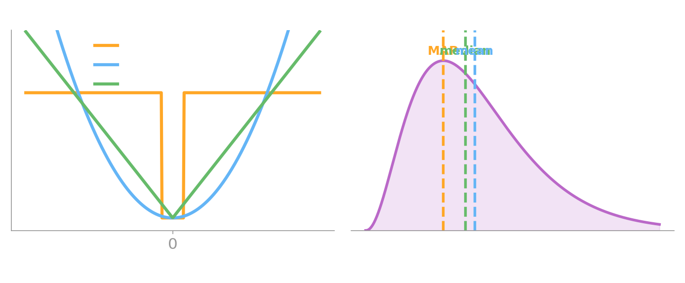
This isn’t a coincidence you have to memorize three times — it’s three readings of “minimize expected loss” against the same posterior. Take a skewed posterior over Chibany’s bento weight and derive each summary by brute force: sweep every candidate estimate, compute its expected loss under the posterior, and keep the cheapest.

 1
 2
 3
 4
 5
 6
 7
 8
 9
10
11
12
13
14
15
16
17
18
19
20
21
22
23

grid = jnp.linspace(0.0, 10.0, 1001)             # candidate weights / estimates (×100 g)
dens = grid**2.3 * jnp.exp(-grid / 1.15)         # a skewed posterior over the weight
dens = dens / jnp.trapezoid(dens, grid)          # normalize it

# the three summaries, read straight off the posterior
mode   = grid[jnp.argmax(dens)]
mean   = jnp.trapezoid(grid * dens, grid)
cdf    = jnp.cumsum(dens) * (grid[1] - grid[0])
median = grid[jnp.argmin(jnp.abs(cdf - 0.5))]
print(f"read off the posterior:   mode = {float(mode):.2f}   mean = {float(mean):.2f}   median = {float(median):.2f}")

# now DERIVE each as the Bayes estimator: the action a minimizing expected loss
def bayes_estimator(loss):
    T, A = grid[None, :], grid[:, None]                       # theta (cols) vs action (rows)
    expected_loss = jnp.trapezoid(loss(T, A) * dens[None, :], grid, axis=1)
    return grid[jnp.argmin(expected_loss)]

a_01  = bayes_estimator(lambda t, a: (jnp.abs(t - a) > 0.05).astype(float))   # 0–1 loss
a_sq  = bayes_estimator(lambda t, a: (t - a) ** 2)                            # squared loss
a_abs = bayes_estimator(lambda t, a: jnp.abs(t - a))                          # absolute loss
print(f"argmin 0–1 loss      = {float(a_01):.2f}   (lands on the mode)")
print(f"argmin squared loss  = {float(a_sq):.2f}   (lands on the mean)")
print(f"argmin absolute loss = {float(a_abs):.2f}   (lands on the median)")

Output:

read off the posterior:   mode = 2.64   mean = 3.70   median = 3.39
argmin 0–1 loss      = 2.62   (lands on the mode)
argmin squared loss  = 3.70   (lands on the mean)
argmin absolute loss = 3.39   (lands on the median)

The three argmins land on the three summaries (the $0$–$1$ result sits on the mode up to the grid’s resolution). For a skewed posterior these are genuinely different numbers — mode $2.64$, median $3.39$, mean $3.70$ — so the loss you pick is not a detail: it moves your answer. The left panel below shows why each loss pulls toward its summary. $0$–$1$ loss pays nothing only when you land within a hair of the truth, so it rewards putting your estimate where the posterior density is highest — the mode (that hair’s-width is the 0.05 tolerance band in the code). The steep parabola of squared loss punishes far-off errors so harshly it chases the mean. And absolute loss, growing at a steady rate, is smallest when you split the posterior mass in half — the median. The right panel marks all three on the posterior:

Click between the loss types yourself and watch the optimal estimate jump between the three summaries — and watch the expected-loss curve below it slide its minimum to match:

(Switch to squared loss and note where the minimum sits; then to absolute, and watch it slide left to the median; then to $0$–$1$, and watch it jump to the peak.)

A Cognitive Aside: the Brain as a Decision Theorist

In GenJAX

Now we can close the loop back to the observation. The threshold rule $d_k$ needed a cutoff $k$, and a cutoff needs the bridge from a day count to a belief about freshness — the days → P(fresh) conversion from the start of the chapter. In GenJAX that conversion is a one-line generative model: the day count sets the freshness probability, and flip draws the hidden state.

1
2
3
4
5
6

from genjax import gen, flip

@gen
def freshness(days):
    p_fresh = 1.0 / (1.0 + jnp.exp((days - 5.0) / 1.5))   # the days -> P(fresh) conversion
    return flip(p_fresh) @ "fresh"                          # True = fresh, False = stale

Now the decision falls out with no new ideas — it’s the Monte-Carlo loop from Chapter 16: for a given day count, sample the freshness many times, average each action’s loss against the table, and take the cheaper. Sweep the days and watch the optimal action flip:

 1
 2
 3
 4
 5
 6
 7
 8
 9
10
11
12

def decide(days, key, n=20000):
    fresh = jax.vmap(lambda k: freshness.simulate(k, (float(days),)).get_retval())(jr.split(key, n))
    f = fresh.astype(float); stale = 1.0 - f
    el_eat     = jnp.mean(f * L[0, 0] + stale * L[1, 0])    # L[theta, action]; action 0 = eat
    el_compost = jnp.mean(f * L[0, 1] + stale * L[1, 1])    # action 1 = compost
    return float(el_eat), float(el_compost)

print(" day  P(fresh)  E[L:eat]  E[L:compost]   decision")
for d in range(8):
    ee, ec = decide(d, jr.fold_in(jr.key(0), d))
    pf = float(1.0 / (1.0 + jnp.exp((d - 5.0) / 1.5)))
    print(f"  {d}      {pf:.2f}     {ee:5.1f}      {ec:5.1f}        {'eat' if ee < ec else 'compost'}")

Output:

 day  P(fresh)  E[L:eat]  E[L:compost]   decision
  0      0.97       0.4        2.9        eat
  1      0.94       0.6        2.9        eat
  2      0.88       1.2        2.8        eat
  3      0.79       2.1        2.6        eat
  4      0.66       3.4        2.3        compost
  5      0.50       5.0        2.0        compost
  6      0.34       6.6        1.7        compost
  7      0.21       7.9        1.4        compost

The decision flips at day 4: eat anything bought in the last three days, compost the rest. That cutoff, $k = 3$, is not a number we picked — it’s what the losses ($10$ for poisoning, $3$ for waste) and the days→freshness model together force, found by nothing more than drawing samples and averaging loss. The abstract threshold rule $d_k$ from the start of the chapter just got its $k$.

This is the same loop you’ll run for the rest of the course. But it raises a question we’ve quietly dodged: each decision drew 20,000 samples. What if each sample costs something?

How Many Samples? One and Done

Drawing twenty thousand samples to decide one lunch is absurd if each sample is a second of thought. Real agents — people, animals, a robot on a deadline — pay for every sample in time, and time spent deliberating is time not spent on the next decision. So the question stops being “how do I get the best estimate?” and becomes “how good a decision can I afford?”

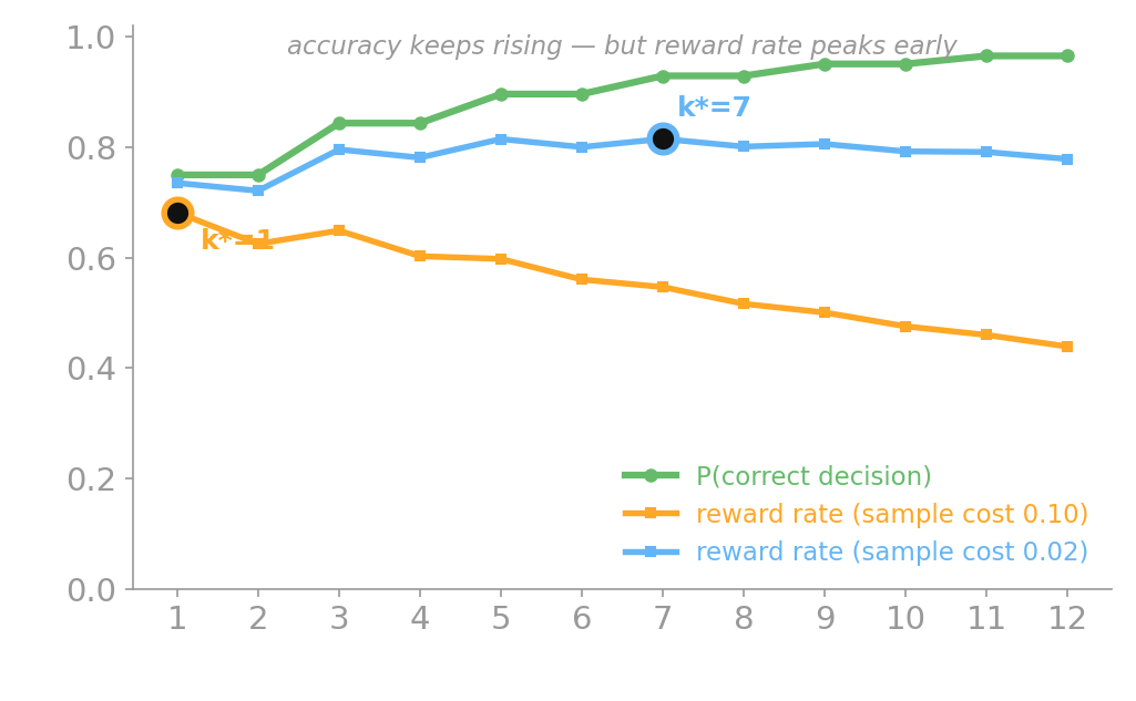
Vul, Goodman, Griffiths & Tenenbaum (2014) made this precise in a paper with a title that gives away the answer: One and Done?. Picture a stream of decisions where, for each, you draw $k$ samples from your belief and go with the majority vote. More samples means a more reliable choice — but the thing you actually want to maximize is your reward rate: good decisions per unit time. If each sample costs time, that rate is

where $c$ is the time cost of one sample relative to the rest of a decision. The accuracy in the numerator rises with $k$; the time in the denominator rises too. (We assume your belief is calibrated — a single sample points to the better option with probability exactly $p$ — so “sample from your belief” and “be right with probability $p$” line up; ties at even $k$ are settled by a fair coin.) Where does the rate peak?

 1
 2
 3
 4
 5
 6
 7
 8
 9
10
11

import jax.numpy as jnp
from jax.scipy.special import gammaln

def p_correct(k, p):
    # P(majority of k samples from your belief favors the better option), ties split fairly.
    # p = your belief that the better option really is better.
    j = jnp.arange(k + 1)
    log_choose = gammaln(k + 1.) - gammaln(j + 1.) - gammaln(k - j + 1.)
    pmf = jnp.exp(log_choose + j * jnp.log(p) + (k - j) * jnp.log1p(-p))
    win = (j > k / 2) + 0.5 * (j == k / 2)
    return float(jnp.sum(pmf * win))

 1
 2
 3
 4
 5
 6
 7
 8
 9
10
11
12
13
14
15

p, cost = 0.75, 0.1               # belief: 75% sure; each sample costs 0.1 of a decision's time
ks   = list(range(1, 13))
acc  = [p_correct(k, p) for k in ks]
rate = [a / (1 + cost * k) for a, k in zip(acc, ks)]
best = ks[int(jnp.argmax(jnp.array(rate)))]

print(" k   P(correct)   reward rate")
for k, a, r in zip(ks, acc, rate):
    print(f"{k:2d}     {a:.3f}        {r:.3f}{'   <- best' if k == best else ''}")
print(f"\noptimal number of samples: k* = {best}  (one and done)")

# what the k=1 policy actually DOES: it follows its single sample, so it picks the
# option it believes is better with probability p -- it MATCHES its belief.
print(f"one-and-done picks the believed-better option with prob {p:.2f}  (probability matching)")
print(f"'always pick the more likely' (maximizing) would pick it with prob 1.00")

Output:

 k   P(correct)   reward rate
 1     0.750        0.682   <- best
 2     0.750        0.625
 3     0.844        0.649
 4     0.844        0.603
 5     0.896        0.598
 6     0.896        0.560
 7     0.929        0.547
 8     0.929        0.516
 9     0.951        0.501
10     0.951        0.476
11     0.966        0.460
12     0.966        0.439

optimal number of samples: k* = 1  (one and done)
one-and-done picks the believed-better option with prob 0.75  (probability matching)
'always pick the more likely' (maximizing) would pick it with prob 1.00

One sample. When thinking costs time, the reward-rate-optimal policy is to draw a single sample from your belief and act on it — one and done. (Notice that an even number of samples never beats the odd one below it — a second sample can only create ties, never break the first — so $k=2$ ties $k=1$ on accuracy but loses on time. Only if samples were nearly free would you draw more: the picture shows the peak sliding right as $c$ shrinks.)

Here is the punchline that makes this a chapter about minds. A one-sample decision picks “fresh” with probability equal to your belief, $0.75$ — it matches the posterior instead of always taking the more likely option. That behavior, probability matching, is one of the oldest “irrationalities” in the psychology of choice: people pick options in proportion to their probability rather than always going with the best one. One and Done reframes it as optimal — exactly what a sampler that values its time should do. The same thread runs through Chapter 19: a mind that reasons from a few samples isn’t a broken Bayesian, it’s an efficient one.

This is the seam where decision theory, Monte Carlo, and cognition meet — and it launches the rest of the course. The next two chapters keep the “decide by sampling your model” loop but stretch the single action into a sequence, where today’s choice changes tomorrow’s world and reward rate becomes the very thing an agent learns to maximize.

Exercises

A companion notebook works through all of this interactively:

📓 Open in Colab: 20_statistical_decision_theory.ipynb

References

• Körding, K. P., & Wolpert, D. M. (2004). Bayesian integration in sensorimotor learning. Nature, 427(6971), 244–247. https://doi.org/10.1038/nature02169
• Vul, E., Goodman, N. D., Griffiths, T. L., & Tenenbaum, J. B. (2014). One and done? Optimal decisions from very few samples. Cognitive Science, 38(4), 599–637. https://doi.org/10.1111/cogs.12101

Special thanks to JPPCA for their generous support of this tutorial series.