Inverse RL: Reading Goals from Behavior

Running the Camera Backwards

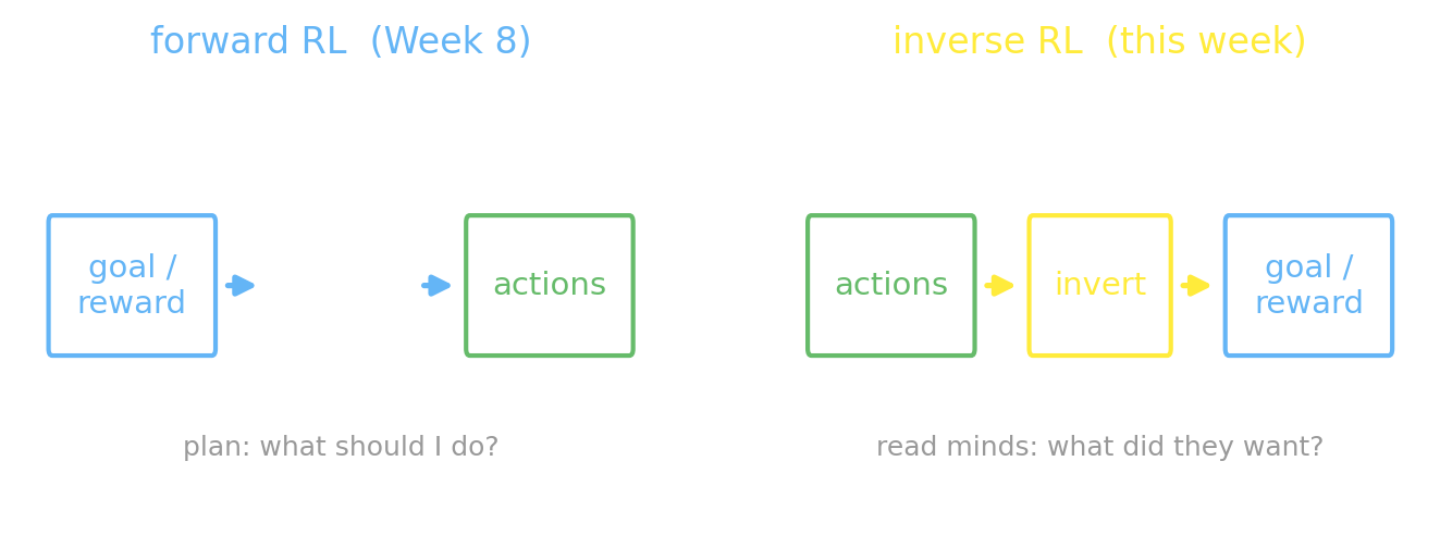
The last three chapters all ran the same direction. A goal (or a reward) defined an MDP; value iteration turned it into a value; the value became a policy; the policy produced actions. Goal → behavior. That direction — forward planning — is what Chapters 20–22 built: even when the model is unknown, Chapter 22’s Q-learning still learns the goal-driven policy.

Now watch the arrow turn around. You see someone in a café get up, walk past the pastry case, past the coffee bar, and straight to the door. You instantly form a belief: they’re leaving. You never saw their goal — you saw three footsteps and ran the planner backwards, asking which goal would have made those footsteps sensible.

Alyssa: “It’s the same machinery, isn’t it? Last week the goal was the input and the actions were the output. Now the actions are the data and the goal is the unknown.”

Jamal: “Right. Freeze a video of someone halfway across a room and you’ll happily bet on where they’re headed. You’re not running their legs — you’re running their plan, in reverse.”

That is inverse reinforcement learning (inverse RL): given behavior, recover the objective behind it. Pose it as a question about a goal and it is goal inference; pose it about a whole reward function and it is reward learning; pose it about another mind and it is Theory of Mind. This chapter builds all three out of one idea — Bayes’ rule with a planner inside the likelihood — and ends at the modern methods (MaxEnt IRL, GAIL, AIRL) that scale it up.

Goal Inference Is Bayes’ Rule

We have done Bayesian inversion many times: a hidden cause, a likelihood that says how the cause produces data, a prior, and a posterior. Goal inference is exactly that, with the goal as the hidden cause and the agent’s policy as the likelihood:

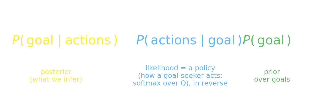
The blue term is the whole trick. $P(\text{actions} \mid \text{goal})$ is not a new object we have to invent — it is the policy a forward planner would follow if it had that goal. Run value iteration for the goal, read off the action values $Q(s,a)$, and turn them into action probabilities with a softmax (defined next): a goal’s policy assigns a probability to every action, which is exactly what a likelihood needs to do.

How do you turn values into probabilities? With the softmax (or Boltzmann) policy:

This says: the best action is the most likely, but every action keeps some probability — a noisy-rational agent, not a perfect one. The new symbol is $\beta \ge 0$, the rationality (or inverse-temperature): it controls how rational. As $\beta \to 0$ the exponent vanishes and every action is equally likely — a coin-flipping agent. As $\beta \to \infty$ the largest $Q$ dominates and the policy becomes greedy — pure exploitation of the best action (not “optimal” in some grander sense, just deterministically greedy). In between, $\beta$ encodes our assumption about how noisily the agent optimizes — “mostly does the smart thing, but slips sometimes” — a knob we choose rather than a property we measure, and that single assumption, as we will see, is what makes a detour informative.

Building the Observer in GenJAX

Let us make it concrete on a tiny world: a $3\times3$ grid. An agent (call it Chibany, padding around a room) starts in the bottom-left and could be heading for any of the three cells along the top — left, mid, or right. We will watch a few moves and infer which.

First the forward planner: deterministic moves, and tabular value iteration run once per candidate goal (entering the goal cell pays $+1$, then the episode ends). This is the Chapter 21 solver, reused unchanged.

 1
 2
 3
 4
 5
 6
 7
 8
 9
10
11
12
13
14
15
16
17
18
19
20
21
22
23
24
25
26
27
28
29

import jax.numpy as jnp
from jax import random
from genjax import gen, categorical, ChoiceMap

NROWS, NCOLS, NA = 3, 3, 4
NS = NROWS * NCOLS
START = 0                                   # (0,0) bottom-left
GOALS = {"left": 6, "mid": 7, "right": 8}   # the three top-row cells
NAMES = list(GOALS)
GOAL_STATES = jnp.array([GOALS[g] for g in NAMES])
GAMMA, BETA = 0.9, 3.0                       # discount; rationality beta (chosen, not inferred)
UP, DOWN, LEFT, RIGHT = 0, 1, 2, 3

def step(s, a):                              # deterministic move, clamped at the walls
    r, c = s // NCOLS, s % NCOLS
    r = jnp.clip(jnp.where(a == UP, r + 1, jnp.where(a == DOWN, r - 1, r)), 0, NROWS - 1)
    c = jnp.clip(jnp.where(a == LEFT, c - 1, jnp.where(a == RIGHT, c + 1, c)), 0, NCOLS - 1)
    return r * NCOLS + c

TRANS = jnp.array([[int(step(s, a)) for a in range(NA)] for s in range(NS)])  # T[s,a] -> s'

def q_values_for_goal(goal):                 # value iteration for ONE goal (the forward planner)
    reward = (TRANS == goal).astype(jnp.float32)     # +1 for entering the goal cell
    is_goal = (jnp.arange(NS) == goal)
    V = jnp.zeros(NS)
    for _ in range(50):
        Q = reward + GAMMA * V[TRANS]
        V = jnp.where(is_goal, 0.0, jnp.max(Q, axis=1))
    return reward + GAMMA * V[TRANS]                  # Q_g(s,a), shape (NS, NA)

Now the inversion. Turn each goal’s $Q$-values into softmax logits, write the agent as a GenJAX generative model — draw a goal, then act by that goal’s policy — and recover the posterior by scoring each goal with assess and normalizing. Because there are only three goals, we can enumerate them and get the exact posterior; no approximation.

 1
 2
 3
 4
 5
 6
 7
 8
 9
10
11
12
13
14
15
16
17
18
19
20
21
22
23
24
25
26

LOGITS = BETA * jnp.stack([q_values_for_goal(g) for g in GOAL_STATES])   # (G, NS, NA)
PRIOR = jnp.ones(len(NAMES)) / len(NAMES)                                 # uniform over goals

@gen
def observer(states):                        # the generative model of a goal-seeker
    g = categorical(jnp.log(PRIOR)) @ "goal"             # 1. draw a hidden goal
    for t in range(len(states)):
        categorical(LOGITS[g, states[t]]) @ f"a_{t}"     # 2. act by goal g's softmax policy

def logsumexp(x):
    m = jnp.max(x); return m + jnp.log(jnp.sum(jnp.exp(x - m)))

def goal_posterior(states, actions):         # exact P(goal | actions) by enumerating goals
    states = jnp.asarray(states)
    logp = []
    for g in range(len(NAMES)):
        cm = ChoiceMap.d({"goal": g, **{f"a_{t}": int(actions[t]) for t in range(len(actions))}})
        score, _ = observer.assess(cm, (states,))        # log P(goal, actions)
        logp.append(score)
    return jnp.exp(jnp.array(logp) - logsumexp(jnp.array(logp)))   # normalize -> posterior

def states_visited(start, actions):          # the state at which each action is taken
    s, out = start, []
    for a in actions:
        out.append(int(s)); s = int(step(jnp.array(s), jnp.array(a)))
    return out

The categorical(LOGITS[g, states[t]]) line is the softmax policy: GenJAX’s categorical(logits) internally computes $\text{softmax}(\text{logits})$ and samples from it, so feeding it LOGITS = β·Q makes each action’s probability $\pi(a\mid s)\propto e^{\beta Q(s,a)}$ — exactly the policy from the formula above. Watch Chibany walk right, right, up, up — across the bottom and up the right wall to the top-right cell — and ask where it was headed:

1
2
3
4
5
6

actions = [RIGHT, RIGHT, UP, UP]             # (0,0)->(0,1)->(0,2)->(1,2)->(2,2): the right goal
states = states_visited(START, actions)
post = goal_posterior(states, actions)
print("observed actions:", ["UP DOWN LEFT RIGHT".split()[a] for a in actions])
for name, p in zip(NAMES, post):
    print(f"  P({name:5s} | actions) = {float(p):.3f}")

Output:

observed actions: ['RIGHT', 'RIGHT', 'UP', 'UP']
  P(left  | actions) = 0.173
  P(mid   | actions) = 0.284
  P(right | actions) = 0.544

The posterior lands on right at $0.54$ — but notice it is not certain, and it leaves real mass on mid ($0.28$). That hedging is correct: walking right is strong evidence against the left goal (which sits up and to the left), but the mid goal is still partly consistent — an agent aiming for the middle-top cell also moves right in its first steps before turning up. The model is uncertain exactly where a thoughtful observer would be.

The Freeze-Frame Curve

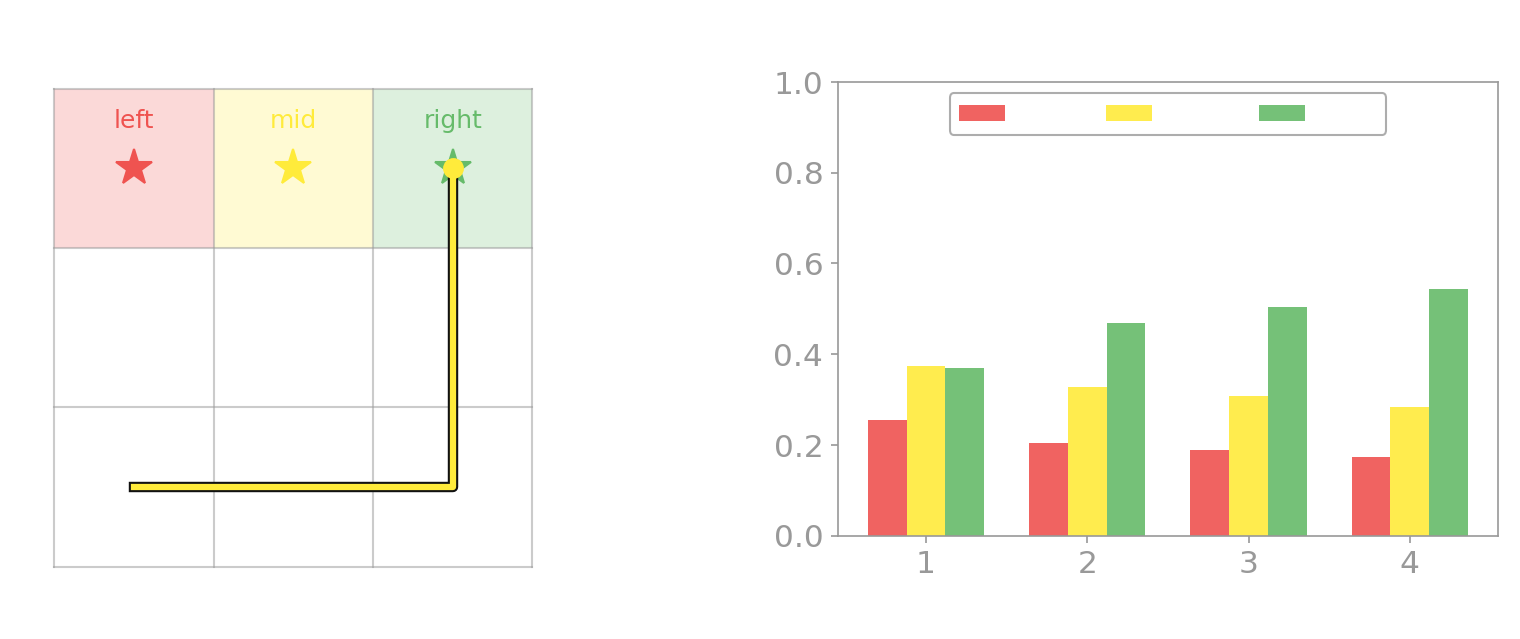
The real charm of goal inference is that it updates as the behavior unfolds. Freeze the video after one step, two steps, three — and recompute. This is the classic experiment of Baker, Saxe & Tenenbaum (2009): show people a partial path and ask where the agent is going.

1
2
3
4

print("step  " + "  ".join(f"{n:>5s}" for n in NAMES))
for k in range(1, len(actions) + 1):
    pk = goal_posterior(states[:k], actions[:k])
    print(f" {k:>2d}   " + "  ".join(f"{float(x):.3f}" for x in pk))

Output:

step   left    mid  right
  1   0.256  0.374  0.370
  2   0.204  0.327  0.469
  3   0.190  0.307  0.503
  4   0.173  0.284  0.544

After one rightward step the model can barely separate mid from right ($0.37$ each) — both want you to move right early — and left is already dipping, because a left-goal agent would have started up-and-left. Each further step that keeps committing rightward pumps probability toward right. The belief slides smoothly as the evidence accrues, rather than flipping all at once — and that smoothness is the softmax at work: because $\beta$ is finite, every goal keeps a little probability of every action, so each step narrows the posterior instead of eliminating a goal outright. That gradualness is the signature of rational goal inference, and it matches how people actually revise their guesses frame by frame.

Drive it yourself. The widget below is the same gridworld; move the agent (or let it walk) and watch the posterior bars respond to every step — including the “freeze partway and guess” interaction:

If the widget doesn’t load: it is the same $3\times3$ grid; you move the agent one step at a time (or let it walk), and the bars show $P(\text{goal}\mid\text{actions so far})$ updating after every move — the freeze-frame curve, live.

Why Inversion Is Ill-Posed (and What Saves It)

Here is the catch that makes inverse RL deep rather than mechanical. The inverse problem is ill-posed: many different goals — many different rewards — can explain the very same behavior. A flat reward of zero everywhere makes every policy optimal — with no reward to chase, every action ties at $Q(s,a)=0$, so nothing is preferred — and it “explains” any path at all. The same holds more generally: adding a constant to a reward, or reshaping it in value-preserving ways (the potential-shaping trick from Chapter 22), leaves the optimal policy untouched, so behavior cannot tell those rewards apart. Walking to the door is consistent with “wants to leave,” “wants to avoid the barista,” and “enjoys walking toward doors.” Behavior alone does not pin down the objective.

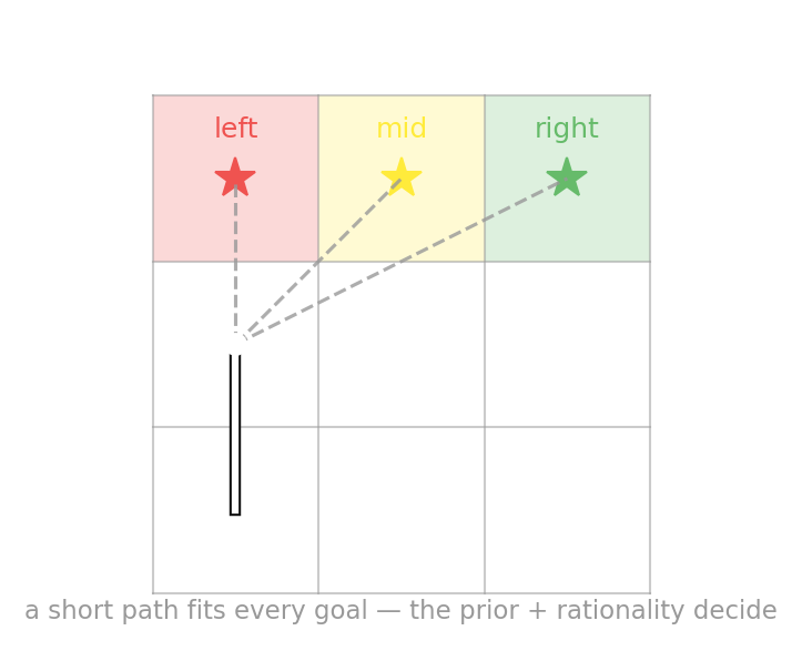
Two things rescue it, and they are exactly the two non-data terms in Bayes’ rule:

• The prior $P(\text{goal})$. We do not entertain every conceivable reward; we put mass on a few plausible goals (the three cells, here). The prior is doing real disambiguating work — a fact worth saying out loud, because it is the most common place students mislocate the “magic.” The data narrows a sensible prior; it does not conjure structure from nothing.
• The rationality assumption $\beta$. Believing the agent is trying — noisily optimizing some reward — is what lets a detour carry information. If you watch someone take the long way around a fence to reach a bench, a rational-agent model concludes the bench must be worth the detour; a coin-flipping model concludes nothing. The more rational you assume the agent is, the more diagnostic its every move. Crucially, $\beta$ is not read off the data — it is a modeling assumption we bring to the inversion, and choosing it badly is its own way for the inference to go wrong.

Turn the rationality knob and watch the same path become more or less informative:

1
2
3
4
5

for b in (0.1, 3.0, 8.0):
    LOGITS = b * jnp.stack([q_values_for_goal(g) for g in GOAL_STATES])
    pk = goal_posterior(states, actions)
    tag = {0.1: "near-random", 3.0: "noisy-rational", 8.0: "near-greedy"}[b]
    print(f"beta={b:>4} ({tag:>14}):  " + "  ".join(f"P({n})={float(x):.3f}" for n, x in zip(NAMES, pk)))

Output:

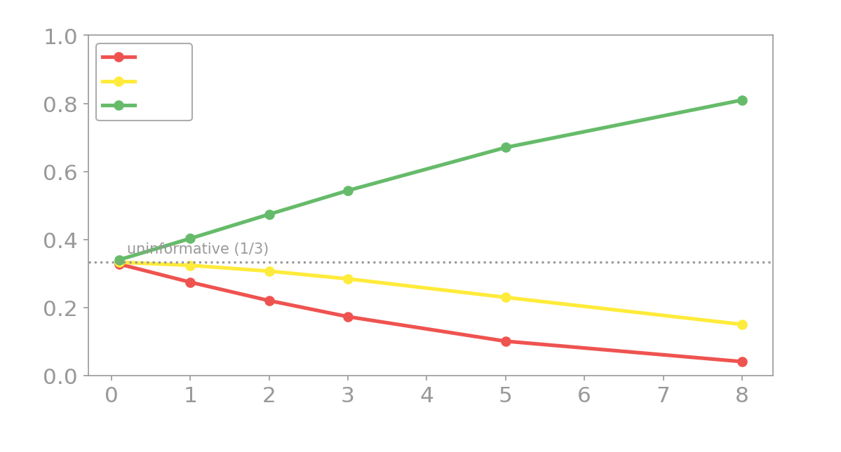
beta= 0.1 (   near-random):  P(left)=0.327  P(mid)=0.333  P(right)=0.340
beta= 3.0 (noisy-rational):  P(left)=0.173  P(mid)=0.284  P(right)=0.544
beta= 8.0 (   near-greedy):  P(left)=0.040  P(mid)=0.150  P(right)=0.810

At $\beta=0.1$ the agent is barely trying, so the path tells us almost nothing — the posterior stays near the uniform prior. At $\beta=8$ we assume near-perfect optimization, so the same rightward commitment becomes damning evidence and the posterior leaps to $0.81$ on right. The rationality you assume sets how much you read into behavior — and choosing $\beta$ badly is one way inverse RL goes wrong.

Theory of Mind Is Inverse RL

Step back and notice what we just built. We took another agent’s behavior and recovered the hidden goal in its head. That is Theory of Mind — and the computational claim of this chapter is that Theory of Mind is inverse RL: reading a mind is inverting a planner. The two are the same computation — both condition on observed behavior to update a posterior over an unobserved cause, using Bayes’ rule with a forward planner inside the likelihood; only the name of the cause changes (a “goal” to a roboticist, a “desire” to a psychologist).

What “Theory of Mind” means in psychology. The phrase comes from comparative and developmental psychology. Premack & Woodruff (1978) coined it for the capacity to attribute mental states — beliefs, desires, goals — to others in order to explain and predict their behavior. The sharpest test of it is the false-belief task: can you represent a belief you know to be false? Its classic form is the Sally-Anne task (Baron-Cohen, Leslie & Frith 1985): Sally hides a marble in a basket and leaves the room; while she is gone, Anne moves it to a box; the child is asked where will Sally look for her marble? Reality says “the box,” but Sally’s belief says “the basket” — answering correctly means holding a belief that differs from the world, and children reliably pass only around age 4. A harder, nested version is the faux-pas test: recognizing a social gaffe means tracking two mental states at once — the speaker’s false belief (they didn’t know it was a secret) plus the listener’s knowledge of how the remark would land. That is a second-order false belief (a belief about a belief), and it is passed years later, around age 9–11. Hold onto that nesting: it returns in Chapter 25, where the faux-pas structure is exactly what large language models are tested on.

This framing comes from Baker & Tenenbaum’s inverse-planning program (Baker, Tenenbaum & Saxe 2007; Baker, Saxe & Tenenbaum 2009), later extended to jointly infer beliefs and desires (Baker et al. 2017) and reviewed under the banner “Theory of Mind as inverse reinforcement learning” by Jara-Ettinger (2019). The attribution matters: the framework is Baker & Tenenbaum’s; Jara-Ettinger’s contribution is the synthesis and the developmental “naïve utility calculus” — children reasoning about others as agents who trade off costs against rewards.

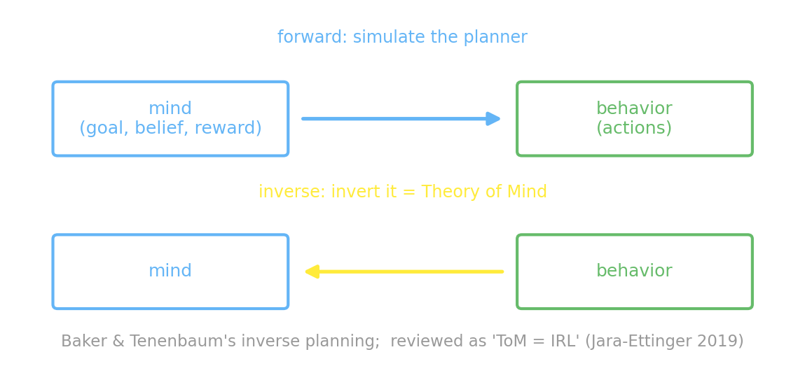
The very same posterior we computed — $P(\text{goal}\mid\text{actions})$ — is, read one way, a planning calculation and, read another, an act of mind-reading. There is one piece still missing, though: so far the agent could see everything. Real minds also hold beliefs that can be wrong, and inferring those is the job of the next chapter — inverting a partially observable MDP. The unifying frame to carry forward is that every one of these inferences asks the same question — which world (which MDP) are we in? — and conditions behavior on observations to answer it.

Recovering the Whole Reward: IRL at Scale

Goal inference picks one cell out of three. The grown-up version recovers an entire reward function over a large or continuous space — and there the ill-posedness bites hard, because now infinitely many rewards fit. What follows is a map of the frontier, not a from-scratch build like the sections above — read it for the lay of the land, and note where the throughline continues in code (Chapter 25 builds the preference-based version, RLHF). Three landmark methods, each adding an assumption to pin one reward down:

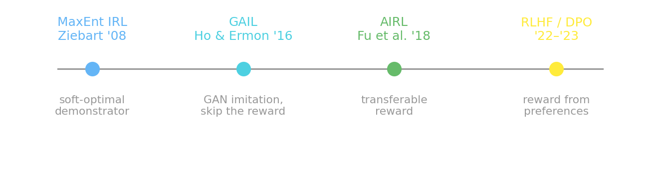
• Maximum-entropy IRL (Ziebart 2008) confronts the ill-posedness head-on. Among all reward-consistent trajectory distributions, it picks the one of maximum entropy — the least committal explanation, assuming no more structure than the data forces. That single principle yields a well-defined reward by maximum likelihood, with trajectory probability $P(\tau)\propto e^{\text{reward}(\tau)}$ — the same softmax-over-value form we used above, now over whole trajectories. MaxEnt IRL is the bridge from this chapter’s toy inversion to deep, scalable reward learning.
• GAIL (Generative Adversarial Imitation Learning; Ho & Ermon 2016) sets up a contest between two learners. A critic learns to tell the expert’s behavior apart from the imitator’s; the imitator keeps adjusting until the critic can no longer tell them apart — at which point the imitator’s behavior is statistically indistinguishable from the expert’s. (This is a GAN, if you have seen them.) It scales imitation to high-dimensional control — but it skips recovering a reward, so there is no transferable objective to hand to a new task.
• AIRL (Adversarial IRL; Fu et al. 2018) keeps the same critic-versus-imitator contest but structures the critic so that a transferable reward falls out of it, disentangled from the environment’s dynamics — combining GAIL’s scale with a reward you can re-optimize in a changed world.

The honest caveat from our toy carries all the way up: a recovered reward is one explanation among many. MaxEnt’s entropy principle and AIRL’s disentanglement are regularizers that pick a reward, not the reward.

You can feel the ill-posedness directly. In the widget below you paint a true reward — click cells to cycle each between $+1$, $0$, and $-1$ — then add demonstrations of an agent that seeks the $+1$ cells and routes around the $-1$ ones. The middle panel recovers a reward from those demonstrations (MaxEnt-style: reward $\propto$ where the agent is drawn versus where it avoids). Watch it light up the goals — and also light up cells that are merely on the way, which it cannot cleanly distinguish from truly rewarded ones. That fuzziness is not a bug in the widget; it is the ill-posedness:

If the widget doesn’t load: paint a true reward on a grid (click cells to cycle $+1$ / $0$ / $-1$), add demonstrations of an agent that seeks the $+1$ cells, and the middle panel recovers an inferred reward — which lights up the true goals and the neutral cells merely on the way to them, making the ill-posedness visible.

This “recover the objective from behavior” thread runs straight into the rest of the unit. Chapter 24 adds hidden beliefs (and then flips the inversion into teaching — acting so you are easy to read). Chapter 25 scales it to the frontier, where RLHF turns human preferences into a reward model — preference-based inverse RL, the same idea that aligns today’s large language models.

Exercises

A companion notebook works through all of this interactively:

📓 Open in Colab: 23_inverse_rl_goal_inference.ipynb

References

• Baker, C. L., Tenenbaum, J. B., & Saxe, R. R. (2007). Goal inference as inverse planning. Proceedings of the 29th Annual Conference of the Cognitive Science Society, 779–784.
• Baker, C. L., Saxe, R., & Tenenbaum, J. B. (2009). Action understanding as inverse planning. Cognition, 113(3), 329–349. https://doi.org/10.1016/j.cognition.2009.07.005
• Baker, C. L., Jara-Ettinger, J., Saxe, R., & Tenenbaum, J. B. (2017). Rational quantitative attribution of beliefs, desires and percepts in human mentalizing. Nature Human Behaviour, 1(4), 0064. https://doi.org/10.1038/s41562-017-0064
• Baron-Cohen, S., Leslie, A. M., & Frith, U. (1985). Does the autistic child have a “theory of mind”? Cognition, 21(1), 37–46. https://doi.org/10.1016/0010-0277(85)90022-8
• Fu, J., Luo, K., & Levine, S. (2018). Learning robust rewards with adversarial inverse reinforcement learning. International Conference on Learning Representations (ICLR). https://arxiv.org/abs/1710.11248
• Ho, J., & Ermon, S. (2016). Generative adversarial imitation learning. Advances in Neural Information Processing Systems (NeurIPS), 29. https://arxiv.org/abs/1606.03476
• Jara-Ettinger, J. (2019). Theory of mind as inverse reinforcement learning. Current Opinion in Behavioral Sciences, 29, 105–110. https://doi.org/10.1016/j.cobeha.2019.04.010
• Ng, A. Y., & Russell, S. J. (2000). Algorithms for inverse reinforcement learning. Proceedings of the 17th International Conference on Machine Learning (ICML), 663–670.
• Premack, D., & Woodruff, G. (1978). Does the chimpanzee have a theory of mind? Behavioral and Brain Sciences, 1(4), 515–526. https://doi.org/10.1017/S0140525X00076512
• Ziebart, B. D., Maas, A., Bagnell, J. A., & Dey, A. K. (2008). Maximum entropy inverse reinforcement learning. Proceedings of the 23rd AAAI Conference on Artificial Intelligence, 1433–1438.

Special thanks to JPPCA for their generous support of this tutorial series.