Markov Decision Processes: Planning When You Know the World

From One Decision to a Sequence

Chapter 20 taught Chibany to make one good decision: weigh the loss, average over the belief, act. But life is not one decision. Eating the bento changes how hungry he is tomorrow; skipping the gym today makes going tomorrow harder. Actions reshape the world that the next action faces. The moment choices have consequences that ripple forward, “pick the best action” is no longer enough — you have to pick the best sequence.

Jamal: “Fine, so just plan the whole week at once — Monday eat light, Tuesday gym, Wednesday…”

Alyssa: “Plan every contingency? If there are even a handful of choices each day, the number of week-long plans explodes. And the world is noisy — Wednesday might not go how you scripted it.”

Alyssa has named the real obstacle — but it pays to be precise, because noise is not actually a second problem. Take the decision-theory solution from Chapter 20 seriously and a noisy world doesn’t break the plan; it just means the right object was never a fixed script. The proper solution is a decision rule that says what to do as a function of what actually happens — eat light Monday, and if Wednesday goes badly, adjust. A rule like that already absorbs the noise; a script is brittle only because it threw the observations away.

What that leaves is the obstacle that genuinely bites: cost. There are $|A|^T$ bare action sequences — $4^{30} \approx 10^{18}$ for a month of four-way choices — and a contingent rule, which must map everything observed so far to an action, lives in a space vastly larger still; even scoring one means averaging the risk over every way the future could unfold given every earlier choice. Sequential decision-making is perfectly well-defined — it is just hopeless to optimize head-on.

The rescue is the Markov property from Chapter 13. If the future depends on the past only through the current state — not the whole history — then the best contingent rule needs nothing but the state you’re in right now. That collapses “a mapping from every history to an action” down to a rule from states to actions, called a policy, and the machinery for finding the best one is the Markov Decision Process (MDP). This chapter builds the MDP, then solves it — exactly — for a world whose rules we fully know.

One more ingredient before we start. A reward today is worth more than the same reward in a thousand years, so we won’t simply add future rewards — we’ll discount them. We’ll meet the discount factor $\gamma$ formally below; for now just hold the intuition that the far future counts for less.

MDPs = Markov Chains + Decisions + Rewards

The cleanest way to understand an MDP is to build one, starting from something you already have. In Chapter 13 a Markov chain was a set of states and a single transition matrix $P$ — Chibany’s mood drifting from day to day with no say in the matter. An MDP adds two things to that chain, one at a time:

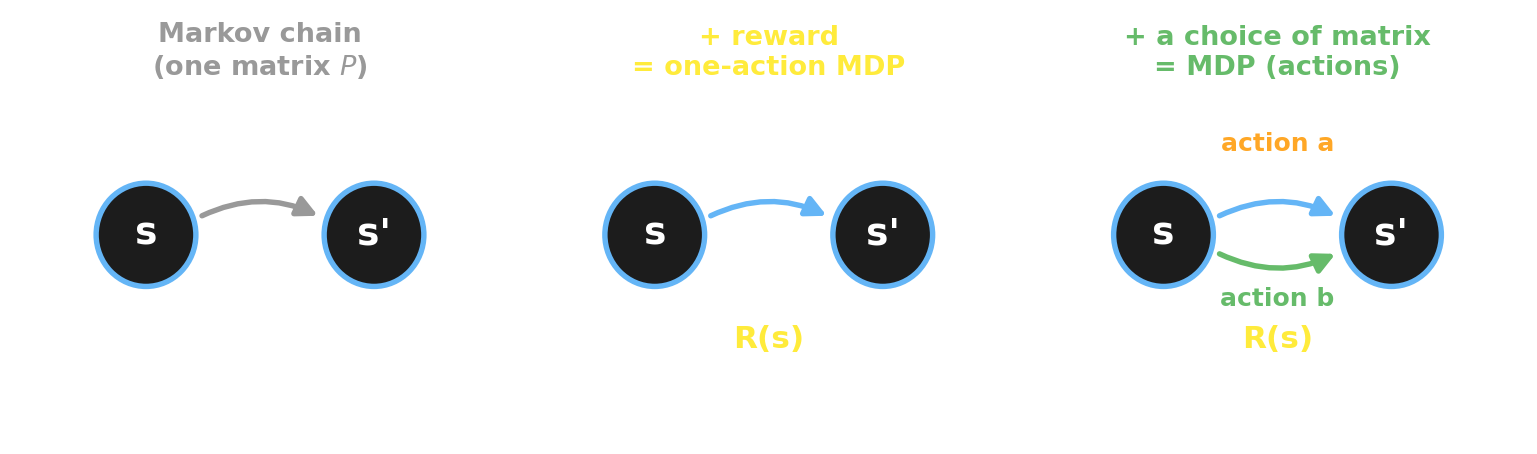
1. Add a reward. Attach a number $R(s)$ to each state — how good it is to be there. A Markov chain with a reward is the simplest possible MDP: a one-action MDP, where you have no choices, you just collect rewards as the chain wanders.
2. Add a choice of the transition matrix. Now give the agent actions. Each action is its own transition matrix: choosing action $a$ means “tomorrow’s state is drawn from this matrix rather than that one.” An action doesn’t set the next state directly — it sets the distribution the next state is drawn from. That is the one idea at the heart of the MDP: an action selects which transition matrix governs tomorrow.

A Markov Decision Process is the five pieces this leaves us with. We name each with its symbol:

• States $S$ — the situations the agent can be in.
• Actions $A$ — the choices available.
• Transition function $T(s' \mid s, a) = P(s_{t+1} = s' \mid s_t = s, a_t = a)$ — one transition matrix per action. (A plain Markov chain is the special case with a single action.)
• Reward $R(s)$ — the payoff in each state. (In general the reward can depend on the action too, $R(s, a)$; Chibany’s depends only on the state.)
• Discount $\gamma \in [0, 1)$ — how much the future is worth relative to now.

And a policy $\pi(a \mid s) = P(a_t = a \mid s_t = s)$ is the agent’s rule: which action to take in each state. Because the world is Markov, a policy needs only the current state — not the history — which is exactly what tames the $|A|^T$ blow-up.

Chibany’s Wellbeing MDP

Make it concrete with the example we’ll carry through the chapter. Chibany’s wellbeing has three states — $0 = $ Junk rut, $1 = $ Trying, $2 = $ Healthy & happy — and two actions: Indulge (order takeout, comfort) or Invest (cook, exercise). The rewards are state-only: $R = [\,+1,\,-2,\,+5\,]$. Junk is mildly pleasant ($+1$); Healthy is great ($+5$); Trying is a trough ($-2$) — effort with no payoff yet.

The whole world is two $3 \times 3$ matrices, one per action — the “action = pick the matrix” idea made literal:

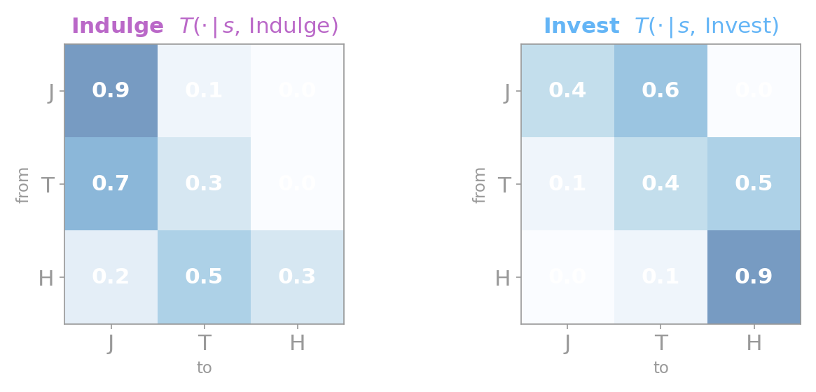
Here is the catch that makes the example worth studying. The only road from Junk to Healthy runs through the $-2$ Trying trough — under Invest, Junk goes to Trying with probability $0.6$. A short-sighted agent stays in the Junk rut collecting $+1$ forever; a far-sighted one swallows the $-2$ to reach the $+5$. Whether Investing is worth it depends entirely on how far ahead Chibany looks — which is exactly what $\gamma$ controls. Hold that thought; it becomes the payoff of the chapter.

In code, the entire MDP is three arrays:

 1
 2
 3
 4
 5
 6
 7
 8
 9
10
11
12
13

import jax
import jax.numpy as jnp
import jax.random as jr
from jax import lax, vmap

# states: 0 = Junk rut, 1 = Trying, 2 = Healthy & happy
# actions: 0 = Indulge, 1 = Invest
T = jnp.array([[[.9, .1, 0.], [.7, .3, 0.], [.2, .5, .3]],     # Indulge: T[0, s, s']
               [[.4, .6, 0.], [.1, .4, .5], [0., .1, .9]]])    # Invest:  T[1, s, s']
R = jnp.array([1., -2., 5.])      # reward of being in each state
gamma = 0.9                       # discount factor
states  = ["Junk", "Trying", "Healthy"]
actions = ["Indulge", "Invest"]

The Transition as a Generative Model

Notice what the transition function is: given a state and an action, it’s a distribution over the next state. That is precisely a generative model of the kind you’ve been writing since Tutorial 2 — and writing it in GenJAX makes the “action picks the distribution” idea executable. The action indexes which row of which matrix to sample from:

 1
 2
 3
 4
 5
 6
 7
 8
 9
10
11
12
13

from genjax import gen, categorical

@gen
def transition(s, a):
    # categorical takes log-probabilities; row T[a, s] is the next-state
    # distribution chosen by action a from state s.
    return categorical(jnp.log(T[a, s])) @ "s_next"

# sample 10,000 next-states from Junk (s=0) under Invest (a=1); should match T[1,0]
draws = vmap(lambda k: transition.simulate(k, (0, 1)).get_retval())(jr.split(jr.key(0), 10000))
freqs = [round(float((draws == j).mean()), 2) for j in range(3)]
print("Junk + Invest -> next-state frequencies:", freqs)
print("the model row T[Invest, Junk]          :", [float(x) for x in T[1, 0]])

Output:

Junk + Invest -> next-state frequencies: [0.41, 0.59, 0.0]
the model row T[Invest, Junk]          : [0.4000000059604645, 0.6000000238418579, 0.0]

The simulated frequencies match the matrix row, as they must. This transition model is the spine of the whole chapter: value iteration will read its probabilities to plan exactly, and at the end we’ll sample from it to plan by simulation — the same generative function, used two ways.

Value, and the Bellman Equation

To choose actions we need to score them, and the score is long-run discounted reward. Three definitions, each symbol named as it arrives:

• The return from time $t$ is the discounted sum of all future rewards, $G_t = R_{t} + \gamma R_{t+1} + \gamma^2 R_{t+2} + \cdots = \sum_{k \ge 0} \gamma^k R_{t+k}$, where $R_t = R(s_t)$ is the reward of the state you’re in at time $t$. The discount $\gamma$ makes this sum finite and makes near rewards count more.
• The state value under a policy $\pi$ is the return you expect by following $\pi$ from state $s$: $v_\pi(s) = \mathbb{E}_\pi[\,G_t \mid s_t = s\,]$. (Because the horizon is infinite and the dynamics don’t change over time, this depends only on which state $s$ you’re in, not on when you’re there.)
• The action value (or Q-value) is the return from taking action $a$ now, then following $\pi$: $q_\pi(s, a) = \mathbb{E}_\pi[\,G_t \mid s_t = s,\, a_t = a\,]$.

The optimal policy $\pi^*$ is the one with the highest value in every state — and one fact makes it simple: the optimal policy is deterministic. (Why? Mixing in any action worse than the best one can only lower the average, so a policy that puts all its weight on the single best action in each state is at least as good as any stochastic one.) So in each state you just take the best action, and the average-over-the-policy $\mathbb{E}_\pi$ collapses into a $\max$ over actions. That gives the Bellman equation — the value of a state is this step’s reward plus the discounted value of wherever you land next:

The bracketed quantity is exactly the action value $q^*(s, a)$ we just defined, so the Bellman equation is simply $v^*(s) = \max_a q^*(s, a)$ — the value of a state is the value of its best action. Read in words: the best you can do from $s$ is the action whose immediate reward plus discounted next-state value is largest. The backup, in one picture:

graph LR
    S["state s"] -->|"each action a"| Q["q*(s,a) = R(s) + γ · expected v* of next state"]
    Q -->|"keep the best"| V["v*(s) = max over a"]
    classDef node fill:none,stroke:#9bbcff,stroke-width:2px,color:#fff
    class S,Q,V node
    linkStyle default stroke:#9bbcff,stroke-width:2px,color:#fff

The equation is recursive — $v^*$ sits on both sides — which looks circular, but the next section turns that self-reference into an iteration that builds $v^*$ up from nothing. That recursion is what makes the problem solvable by dynamic programming, instead of by enumerating $|A|^T$ plans.

Value Iteration

The Bellman equation is a fixed point: plug the right $v^*$ into the right side and the same $v^*$ comes out. Value iteration finds that fixed point the obvious way — start with a guess (all zeros), apply the Bellman update over and over, and watch it converge:

Each sweep “backs up” value one step further from the future. In JAX the whole algorithm is a Bellman operator and a scan:

 1
 2
 3
 4
 5
 6
 7
 8
 9
10
11

def bellman(V, g=gamma):
    Q = R[None, :] + g * (T @ V)            # Q[a, s] is exactly q(s, a) = R(s) + g * sum_s' T(s'|s,a) V(s')
    return jnp.max(Q, axis=0), jnp.argmax(Q, axis=0)   # max over a -> v(s); argmax over a -> best action

def value_iteration(n_sweeps=300, g=gamma):
    V, _ = lax.scan(lambda V, _: (bellman(V, g)[0], None), jnp.zeros(3), None, length=n_sweeps)
    return V, bellman(V, g)[1]              # converged values, and the greedy policy

Vstar, pistar = value_iteration()
print("V* =", [round(float(v), 1) for v in Vstar])
print("optimal policy:", [actions[int(a)] for a in pistar])

Output:

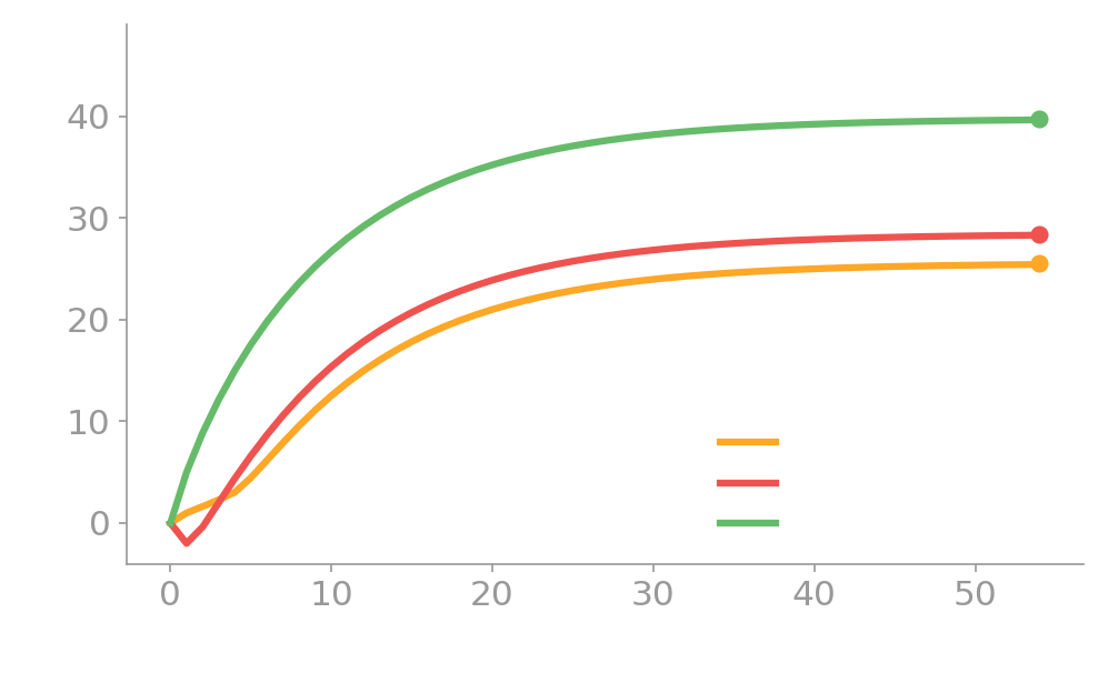
V* = [25.6, 28.4, 39.8]
optimal policy: ['Invest', 'Invest', 'Invest']

At $\gamma = 0.9$, the optimal policy is to Invest in every state — even in the Junk rut, where Investing means walking straight into the $-2$ trough. The values make the gamble legible: $v^*(\text{Junk}) = 25.6$ is far more than the $+1$-per-step Chibany would earn by indulging forever. Knowing the model, value iteration sees all the way to the $+5$ and decides the trough is worth it.

It is worth watching the policy change its mind. Early sweeps see only a few steps ahead, so Junk still prefers the safe $+1$ of Indulge; only once enough value has backed up from Healthy does Junk flip to Invest:

1
2
3
4
5
6

V = jnp.zeros(3)
print("sweep   V(Junk)  V(Trying)  V(Healthy)   Junk's best action")
for k in range(1, 6):
    Vn, pol = bellman(V)
    print(f"  {k}     {float(Vn[0]):6.2f}   {float(Vn[1]):6.2f}    {float(Vn[2]):6.2f}      {actions[int(pol[0])]}")
    V = Vn

Output:

sweep   V(Junk)  V(Trying)  V(Healthy)   Junk's best action
  1       1.00    -2.00      5.00      Indulge
  2       1.63    -0.38      8.87      Indulge
  3       2.29     2.00     12.15      Indulge
  4       3.03     4.39     15.02      Indulge
  5       4.46     6.61     17.56      Invest

Watch Healthy’s $+5$ march leftward through the table, one backup per sweep — that is what “backs up value one step further” means, made concrete. It lifts Trying from $-2$ (sweep 1) up through $+2.00$ (sweep 3); and only once that risen value reaches Junk does the trough finally pay for itself, so on sweep 5 Junk commits to Invest. The values keep climbing for another few hundred sweeps until they settle at $[25.6, 28.4, 39.8]$:

Step through value iteration yourself below — advance it one sweep at a time and watch the value bars fill and the policy arrows settle:

How Far Ahead? The Discount Factor

Everything above used $\gamma = 0.9$ — a far-sighted Chibany. But the whole drama of the Trying trough is about patience: the $-2$ only pays off if you value the $+5$ that comes later. So what happens as we dial $\gamma$ down — as Chibany cares less and less about the future?

1
2
3
4
5
6

gammas = jnp.linspace(0.0, 0.95, 200)
junk_action = jnp.array([value_iteration(300, float(g))[1][0] for g in gammas])   # Junk's best action
flip = float(gammas[int(jnp.argmax(junk_action == 1))])                           # first gamma that picks Invest
print(f"Junk's action flips Indulge -> Invest at gamma ~ {flip:.2f}")
for g in [0.5, 0.6, 0.64, 0.7, 0.9]:
    print(f"  gamma = {g}:  Junk -> {actions[int(value_iteration(300, g)[1][0])]}")

Output:

Junk's action flips Indulge -> Invest at gamma ~ 0.64
  gamma = 0.5:  Junk -> Indulge
  gamma = 0.6:  Junk -> Indulge
  gamma = 0.64:  Junk -> Invest
  gamma = 0.7:  Junk -> Invest
  gamma = 0.9:  Junk -> Invest

There is a sharp threshold at $\gamma \approx 0.64$. Below it, Chibany is too impatient — the discounted $+5$ isn’t worth the $-2$ today, so he stays in the rut and Indulges. Above it, the future is worth enough that he braves the trough and Invests. The same MDP, the same rewards — only how far ahead he looks — decides whether he escapes:

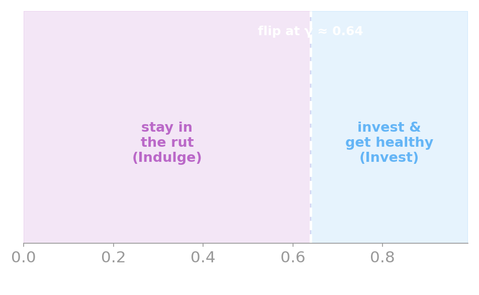
The step plot shows that the policy flips, but not why there. The mechanism is a race between the two action values at Junk — exactly the $q^*(\text{Junk}, a)$ we defined earlier. Plot the advantage of Investing over Indulging, $q^*(\text{Junk}, \text{Invest}) - q^*(\text{Junk}, \text{Indulge})$, against $\gamma$: it is negative for the impatient agent (Indulge is worth more) and crosses zero into positive (Invest is worth more) at exactly $\gamma \approx 0.64$. The flip is that crossing.

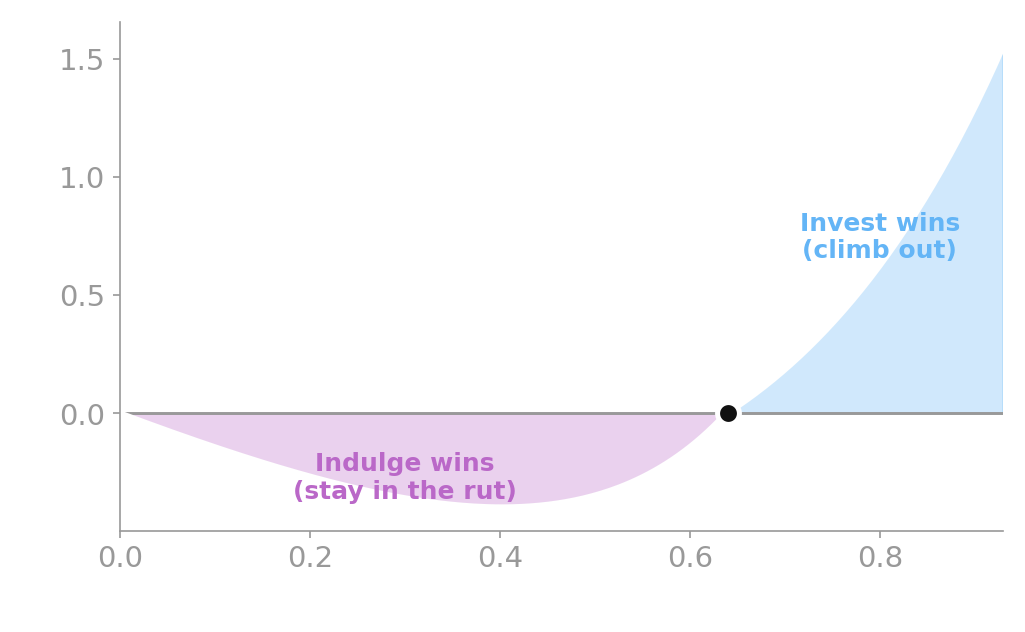
(The value-iteration widget above has a $\gamma$ slider — drag it across $0.64$ and watch Junk’s policy arrow flip.) This is the discounting payoff: a single number, $\gamma$, encoding how patient the agent is, can be the difference between a life stuck in the Junk rut and one that climbs out.

Know the Model → Simulate

Value iteration computed $v^*$ exactly by reading the transition probabilities. But we have the transition as a generative model — so there’s a second way to find a state’s value that needs no Bellman algebra at all: simulate. To roll out a trajectory is to play one possible future forward: start in a state, follow the policy to pick an action, sample the next state from the model, and repeat — collecting the reward of every state you pass through. (“Rolling out” is simply RL’s term for this forward simulation; nothing more.) Estimate a value by rolling out many trajectories from $s$, summing each one’s discounted rewards, and averaging. Nothing about the method has changed — this is exactly the Monte-Carlo estimator from Chapter 16. There you estimated an expectation $\mathbb{E}_P[f(X)]$ by drawing samples $X$ and averaging $f(X)$; here the random sample $X$ is a whole trajectory and the function $f$ is its discounted return $G$. Since a value simply is the expected return, estimating it is the same sample-and-average as before:

Each trajectory is a chain of transition.simulate calls — the same @gen model, now sampled instead of read. The Chibany MDP has no terminal state, so a return is in principle an infinite discounted sum; but $\gamma^{80} \approx 0.0002$, so truncating each rollout at an $80$-step horizon drops only a negligible tail. (The reward at step $0$ is undiscounted — disc starts at $1$ — and each step multiplies in another factor of $\gamma$.)

 1
 2
 3
 4
 5
 6
 7
 8
 9
10
11
12
13
14

def mc_value(s0, policy, key, horizon=80, n_traj=5000):
    def one_trajectory(key):
        def step(carry, _):
            s, disc, total, key = carry
            key, k = jr.split(key)
            s_next = transition.simulate(k, (s, policy[s])).get_retval()   # sample the model
            # credit R for the state we're IN, weighted by disc = gamma^k; then discount and move on
            return (s_next, disc * gamma, total + disc * R[s], key), None
        (_, _, total, _), _ = lax.scan(step, (s0, 1.0, 0.0, key), None, length=horizon)
        return total
    return vmap(one_trajectory)(jr.split(key, n_traj)).mean()              # average over rollouts

vhat = mc_value(0, pistar, jr.key(1))      # value of Junk under the optimal policy, by simulation
print(f"Monte-Carlo V(Junk) = {float(vhat):.1f}   vs exact V*(Junk) = {float(Vstar[0]):.1f}")

Output:

Monte-Carlo V(Junk) = 25.7   vs exact V*(Junk) = 25.6

Simulating five thousand of Chibany’s possible futures and averaging their discounted returns gives $25.7$ — within a whisker of the exact $25.6$.

Watch the rollouts pile up and the running average home in on $v^*$:

This is the punchline: if you know the dynamics, you can sit and simulate the optimal policy — no learning required. Planning, in a known world, is just simulation. It is the bridge to everything that follows.

Exercises

A companion notebook works through all of this interactively:

📓 Open in Colab: 21_markov_decision_processes.ipynb

References

• Hafner, D., Lillicrap, T., Ba, J., & Norouzi, M. (2020). Dream to control: Learning behaviors by latent imagination. International Conference on Learning Representations (ICLR). https://arxiv.org/abs/1912.01603
• Schrittwieser, J., Antonoglou, I., Hubert, T., et al. (2020). Mastering Atari, Go, chess and shogi by planning with a learned model. Nature, 588(7839), 604–609. https://doi.org/10.1038/s41586-020-03051-4
• Silver, D., Hubert, T., Schrittwieser, J., et al. (2018). A general reinforcement learning algorithm that masters chess, shogi, and Go through self-play. Science, 362(6419), 1140–1144. https://doi.org/10.1126/science.aar6404

Special thanks to JPPCA for their generous support of this tutorial series.