POMDPs and Belief: Inferring a Hidden World

When the Agent Can’t See the State

Chapter 23 inferred a hidden goal from behavior. But it quietly assumed the agent itself could see everything — it knew exactly which cell it was in. Real agents are not so lucky. A doctor cannot see the disease, only the symptoms; a robot’s camera is noisy; you cannot see the tiger behind the door. The state is hidden, and the agent must act anyway — interleaving cheap information-gathering with an eventual commitment, never fully certain when it acts.

Jamal: “So now there are two layers of not-knowing. We don’t know the agent’s goal, like last chapter — but also the agent doesn’t know the world it’s in.”

Alyssa: “Right. And the agent’s only handle on that hidden world is a running summary of everything it has seen so far. We’ll give that summary a name — a belief — and watch it do all the work.”

This is a partially observable Markov decision process (POMDP): an MDP whose state you never observe directly, only through noisy observations. This chapter builds the belief update that drives it, uses it to decide when to stop gathering evidence and act, and then — in the second half — flips the whole thing around: if you know someone will infer your goal from your actions, you can choose actions that make your goal easy to read. That is teaching.

The Tiger Behind the Door

The cleanest POMDP in the world is the Tiger problem (Kaelbling, Littman & Cassandra 1998). Two doors. Behind one is a tiger; behind the other, freedom. You don’t know which. You may listen (it costs a little and is only 85% accurate — the growl comes from the right door’s side 85% of the time), open-left, or open-right. Opening the safe door pays $+10$; opening the tiger pays $-100$; a listen costs $-1$.

You cannot see the state $s \in \{\text{tiger-left}, \text{tiger-right}\}$. What you can track is a belief: a probability distribution over the state, given everything you’ve heard,

A belief is not a new kind of object — it is a probability, the posterior over the hidden state. (With only two states we’ll often write the single number $b = b(\text{tiger-left})$ for the whole belief, since $b(\text{tiger-right}) = 1-b$.) Each time you listen, you fold the new growl in with Bayes’ rule, exactly as in the last chapter, but now the hidden cause is the world state rather than a goal:

(In a POMDP where you also move between observations, the update first pushes the belief through the transition dynamics and then folds in the observation; in the Tiger you only listen — nothing moves — so the update is purely observational. The figure further down shows the general form.)

Here is the POMDP and its belief update in GenJAX. The generative model of a single listen is two lines — the hidden state comes from the belief, the growl comes from the state — and the update enumerates the two states and normalizes:

 1
 2
 3
 4
 5
 6
 7
 8
 9
10
11
12
13
14
15
16
17
18
19
20
21
22
23
24

import jax.numpy as jnp
from genjax import gen, categorical, ChoiceMap

# states: 0 = tiger-LEFT, 1 = tiger-RIGHT ; observations: 0 = hear-LEFT, 1 = hear-RIGHT
ACC = 0.85                                          # listening is 85% accurate
OBS = jnp.array([[ACC, 1 - ACC],                    # tiger-left  -> hear-left .85 / right .15
                 [1 - ACC, ACC]])                   # tiger-right -> hear-left .15 / right .85
R_LISTEN, R_CORRECT, R_TIGER = -1.0, 10.0, -100.0   # listen -1, open correct +10, open tiger -100
HEAR_LEFT, HEAR_RIGHT = 0, 1

@gen
def listen(belief):                                 # the generative model of one listen
    s = categorical(jnp.log(belief)) @ "s"          # the hidden state, drawn from the belief
    categorical(jnp.log(OBS[s])) @ "o"              # the growl we actually hear

def update_belief(belief, obs):                     # b'(s) proportional to P(obs|s) b(s)
    logp = jnp.array([listen.assess(ChoiceMap.d({"s": s, "o": int(obs)}), (belief,))[0]
                      for s in range(2)])
    p = jnp.exp(logp - jnp.max(logp))
    return p / jnp.sum(p)

def E_open_right(belief):                            # expected reward of opening the right door
    bL, bR = float(belief[0]), float(belief[1])
    return bL * R_CORRECT + bR * R_TIGER            # +10 if tiger-left, -100 if tiger-right

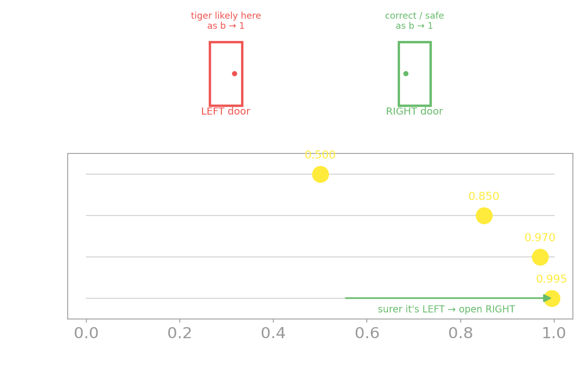
Now start from total ignorance — $b = (0.5, 0.5)$ — and let the tiger keep growling from the left. Watch the belief slide:

1
2
3
4
5

b = jnp.array([0.5, 0.5])                            # uniform prior: no idea which door
print(f"start: P(tiger-left) = {float(b[0]):.4f}")
for k in range(1, 4):
    b = update_belief(b, HEAR_LEFT)                 # the tiger keeps sounding from the left
    print(f"  after {k} left-growl(s): P(tiger-left) = {float(b[0]):.4f}   E[open-right] = {E_open_right(b):+.2f}")

Output:

start: P(tiger-left) = 0.5000
  after 1 left-growl(s): P(tiger-left) = 0.8500   E[open-right] = -6.50
  after 2 left-growl(s): P(tiger-left) = 0.9698   E[open-right] = +6.68
  after 3 left-growl(s): P(tiger-left) = 0.9945   E[open-right] = +9.40

One growl takes you from $0.5$ to $0.85$; a second agreeing growl to $0.97$; a third to $0.99$. The belief slides toward certainty, but never quite arrives — that is the noisy ear at work. Each agreeing growl multiplies the odds by the same likelihood ratio $0.85/0.15 \approx 5.7$: even odds become about $5.7{:}1$ (that’s $b=0.85$), then $32{:}1$ ($b=0.97$). The evidence compounds — which is exactly why one growl leaves you hesitating and two convince you.

When to Stop Listening: α-Vectors

The belief is only half the story. The agent must decide: keep paying $-1$ to listen, or commit to a door? Look back at the E[open-right] column above. It is negative after one growl ($-6.50$) but positive after two ($+6.68$). Somewhere between $b=0.85$ and $b=0.97$, opening the right door becomes worth it.

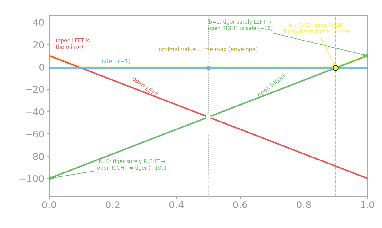
We can find that point exactly. Opening the right door pays $+10$ if the tiger is on the left (probability $b$) and $-100$ if it’s on the right (probability $1-b$), so its expected value is a straight line in the belief:

It is a straight line for a simple reason: an expected value is a weighted average, which is linear in the weights — and the belief is the weights. That line — one per action — is called an α-vector: the value of committing to that action, read as a function of belief. The point of giving it a name is that you can draw all three action-lines once, take their upper envelope (the highest line at each belief = the best action there), and read the entire policy straight off the plot — no re-solving as the belief moves. Opening beats listening (value $-1$) exactly when $110b - 100 > -1$:

1
2
3
4
5
6
7
8
9

# E[open-right] is linear in the belief b = P(tiger-left):  10*b - 100*(1-b) = 110*b - 100.
# It beats listening (-1) when 110*b - 100 > -1, i.e. b > 99/110.
threshold = 99 / 110
print(f"E[open-right] = 110*b - 100   (a straight line in b)")
print(f"opening beats listening when b > {threshold:.4f}")
b1 = update_belief(jnp.array([0.5, 0.5]), HEAR_LEFT)
b2 = update_belief(b1, HEAR_LEFT)
print(f"  1 growl : b = {float(b1[0]):.3f}  ->  below {threshold:.2f}, LISTEN again")
print(f"  2 growls: b = {float(b2[0]):.3f}  ->  above {threshold:.2f}, OPEN the right door")

Output:

E[open-right] = 110*b - 100   (a straight line in b)
opening beats listening when b > 0.9000
  1 growl : b = 0.850  ->  below 0.90, LISTEN again
  2 growls: b = 0.970  ->  above 0.90, OPEN the right door

The threshold is $b = 0.90$ (the $99/110$ above, exactly). One growl ($0.85$) leaves you just short — listen again. A second agreeing growl ($0.97$) clears it — open. Plot all three α-vectors (listen, open-left, open-right) against belief and the optimal value is their upper envelope; its breakpoints are exactly these decision thresholds:

The decision, step by step

Put the belief update and the threshold together and a POMDP policy is a walk along that plot. Start uncertain; each growl slides the belief; when it crosses a threshold, a terminal action’s line rises above “listen” and you commit.

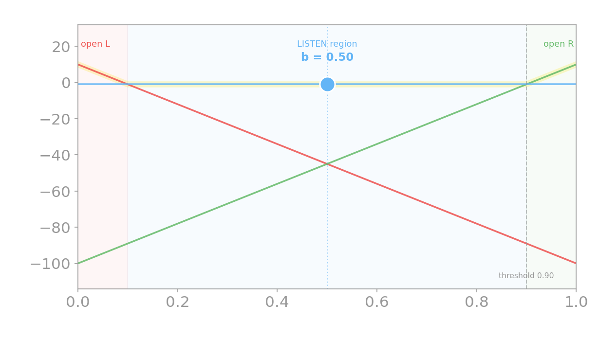
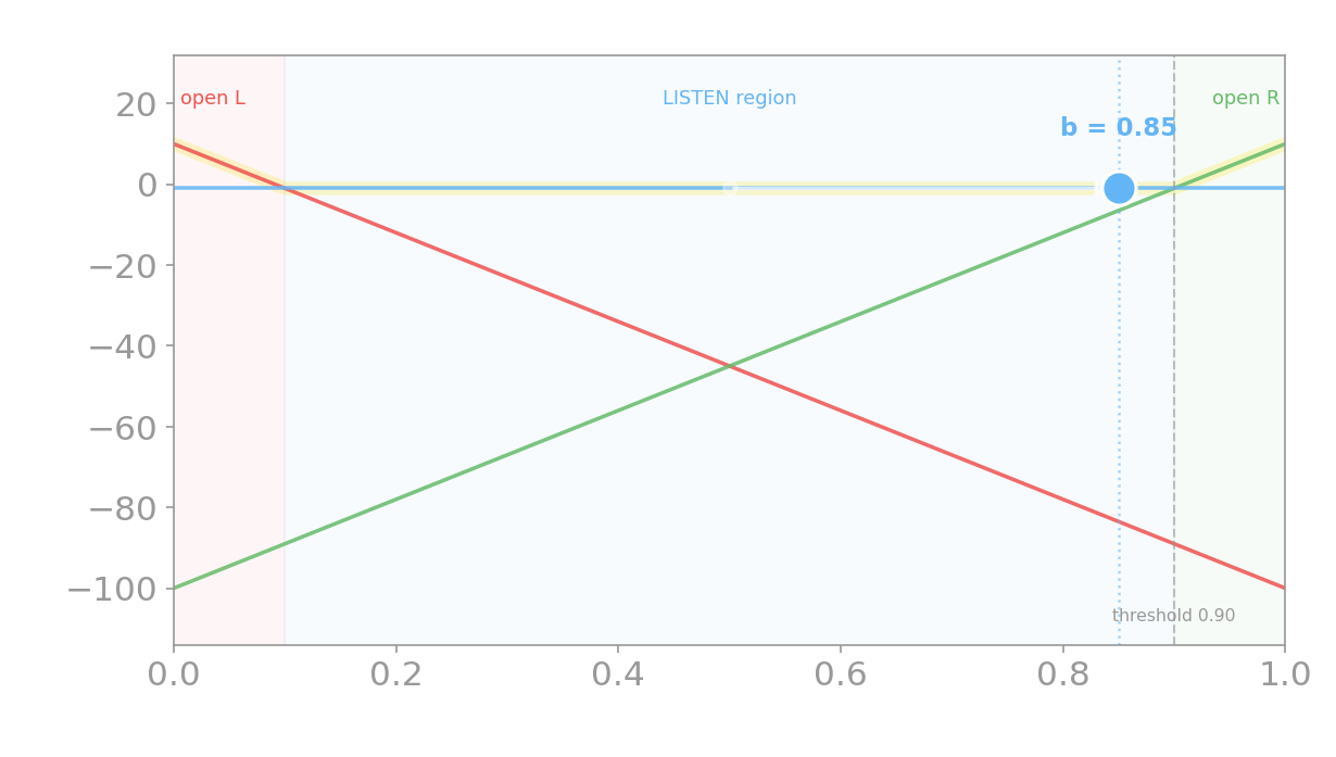
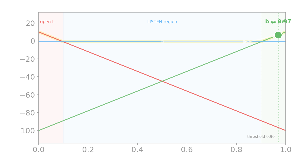
You ride the listen line gathering cheap evidence, until the belief crosses a threshold where a terminal action’s value rises above it — then you act. Drive it yourself; the widget lets you send growls (and adjust the accuracy, costs, and rewards) and watch the belief and the decision move:

If the widget doesn’t load: it is the Tiger tracker — click to send left/right growls, watch $P(\text{tiger-left})$ update and the marker ride the α-vector plot, and drag the sliders for listening accuracy and the listen / open / tiger payoffs to move the decision threshold.

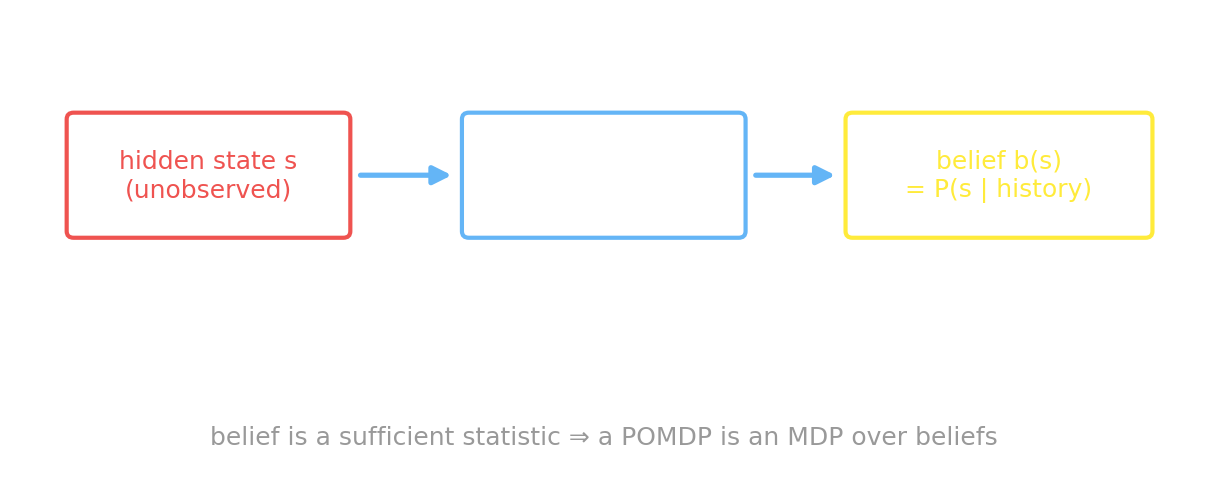
One more sanity check that a belief really is just a probability: contradictory evidence cancels. Hear one growl from each side and you are back where you started.

1
2

b_cancel = update_belief(update_belief(jnp.array([0.5, 0.5]), HEAR_LEFT), HEAR_RIGHT)
print(f"hear-left then hear-right: P(tiger-left) = {float(b_cancel[0]):.4f}")

Output:

hear-left then hear-right: P(tiger-left) = 0.5000

Reading Beliefs in Others

In Chapter 23 we inferred another agent’s goal. Now that agents carry beliefs that can be wrong, Theory of Mind gets a second hidden variable. Bayesian Theory of Mind (Baker, Jara-Ettinger, Saxe & Tenenbaum 2017) inverts a POMDP-planning agent to recover both what it wants and what it believes — and the two trade off.

The classic demonstration is the food-truck experiment. A hungry student walks toward a truck, then stops and detours to a second one. A pure goal-inference model is puzzled — but add a belief, and it explains itself: the student wanted the first truck but believed it might be closed, so they hedged toward the backup. Detours that look irrational under known-state inference become rational once you let the agent be uncertain about the world, exactly like the Tiger.

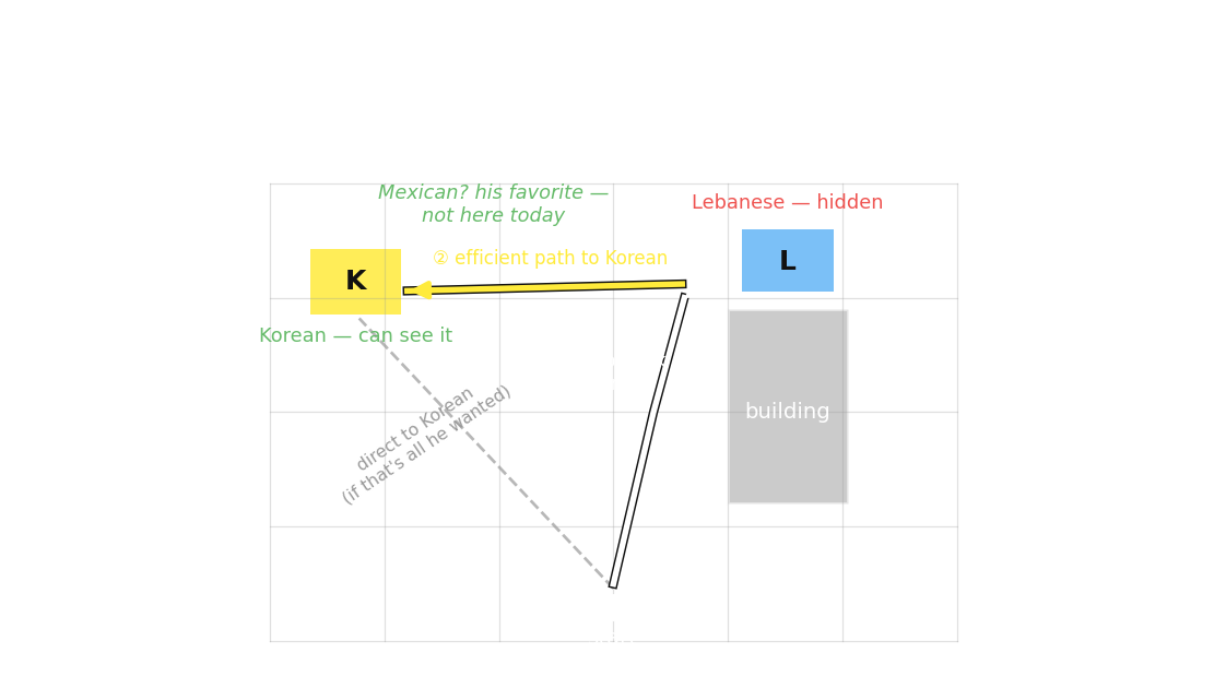
This is the same inversion as before, now over a richer hidden cause. The unifying frame for the whole unit: every one of these inferences asks “which world — which MDP — are we in?” A goal, a belief, a reward — each is a latent we condition observations on to recover.

Flipping the Inversion: Teaching

Here is the turn. Everything so far has been an observer inferring a hidden variable from an agent’s behavior. Now stand in the agent’s shoes and suppose you know you are being inferred. Then you can pick actions not just to reach your goal, but to make your goal legible — easy to read. Why would an agent bother? Because cooperation runs on it: a teacher, a teammate, a robot working beside a person all succeed faster when their intentions are easy to read. Reading minds (the first half of this chapter) and being readable (this half) are the same inversion run in opposite directions. That last move is teaching, and it is inverse planning run one level up: the forward planner asks “what should I do to reach my goal?”; the teacher asks “what should I do so you can tell what my goal is?”

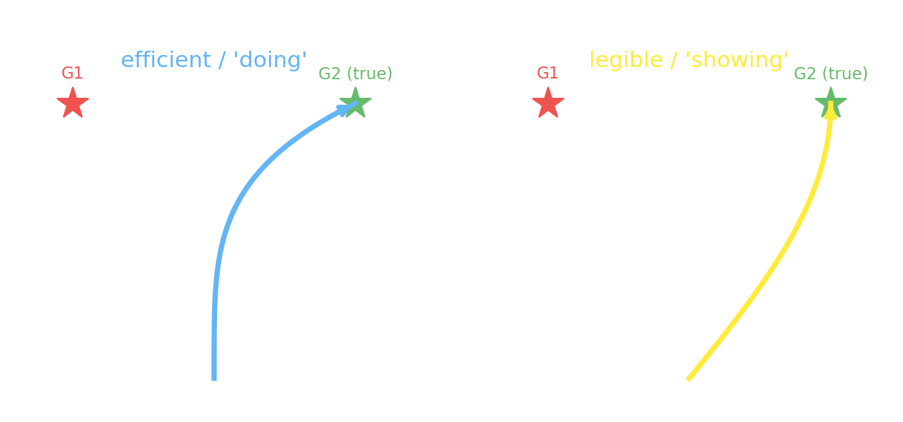
Two paths to the same goal can be the same length yet wildly different in how fast they reveal the goal. Take a grid with two possible goals — top-left and top-right — and an agent heading for the top-right. The efficient (“doing”) path goes straight up the middle and only veers right at the end; the legible (“showing”) path commits right on the first move. Score each by the observer’s posterior on the true goal — reusing the exact inverse-planning machinery from the last chapter:

 1
 2
 3
 4
 5
 6
 7
 8
 9
10
11
12
13
14
15
16
17
18
19
20
21
22
23
24
25
26
27
28
29
30
31
32
33
34
35
36
37
38
39
40
41
42
43
44

NROWS, NCOLS, NA = 3, 3, 4
NS = NROWS * NCOLS
START = 1                                           # (0,1) bottom-middle
GOALS = {"left": 6, "right": 8}                     # top-left / top-right
GNAMES = list(GOALS); GOAL_STATES = jnp.array([GOALS[g] for g in GNAMES])
GAMMA, BETA = 0.9, 3.0
UP, DOWN, LEFT, RIGHT = 0, 1, 2, 3

def step(s, a):
    r, c = s // NCOLS, s % NCOLS
    r = jnp.clip(jnp.where(a == UP, r + 1, jnp.where(a == DOWN, r - 1, r)), 0, NROWS - 1)
    c = jnp.clip(jnp.where(a == LEFT, c - 1, jnp.where(a == RIGHT, c + 1, c)), 0, NCOLS - 1)
    return r * NCOLS + c

TRANS = jnp.array([[int(step(s, a)) for a in range(NA)] for s in range(NS)])

def q_for_goal(goal):
    reward = (TRANS == goal).astype(jnp.float32)
    is_goal = (jnp.arange(NS) == goal)
    V = jnp.zeros(NS)
    for _ in range(50):
        V = jnp.where(is_goal, 0.0, jnp.max(reward + GAMMA * V[TRANS], axis=1))
    return reward + GAMMA * V[TRANS]

LOGITS = BETA * jnp.stack([q_for_goal(g) for g in GOAL_STATES])
GPRIOR = jnp.ones(len(GNAMES)) / len(GNAMES)

@gen
def watcher(states):
    g = categorical(jnp.log(GPRIOR)) @ "goal"
    for t in range(len(states)):
        categorical(LOGITS[g, states[t]]) @ f"a_{t}"

def posterior_true(true_idx, states, actions):      # observer's prob on the TRUE goal
    logp = jnp.array([watcher.assess(
        ChoiceMap.d({"goal": g, **{f"a_{t}": int(actions[t]) for t in range(len(actions))}}),
        (jnp.asarray(states),))[0] for g in range(len(GNAMES))])
    post = jnp.exp(logp - jnp.max(logp)); post = post / jnp.sum(post)
    return float(post[true_idx])

def states_of(start, acts):
    s, out = start, []
    for a in acts: out.append(int(s)); s = int(step(jnp.array(s), jnp.array(a)))
    return out

1
2
3
4
5
6
7
8
9

TRUE = GNAMES.index("right")
doing   = [UP, UP, RIGHT]        # straight up the middle, then over: ambiguous early
showing = [RIGHT, UP, UP]        # commit to the right immediately: legible
print("observer's P(true goal = top-right) after each step:")
print("  step   doing(efficient)   showing(legible)")
for k in range(1, 4):
    pd = posterior_true(TRUE, states_of(START, doing)[:k],   doing[:k])
    ps = posterior_true(TRUE, states_of(START, showing)[:k], showing[:k])
    print(f"   {k}          {pd:.3f}              {ps:.3f}")

Output:

observer's P(true goal = top-right) after each step:
  step   doing(efficient)   showing(legible)
   1          0.500              0.613
   2          0.500              0.647
   3          0.639              0.685

The numbers tell the whole story. After the first move, the efficient path leaves the observer at $0.500$ — dead uncertain, because going straight up is equally consistent with both goals — while the legible path has already lifted the observer to $0.613$, because a rightward first step is something an agent aiming for the left goal would almost never take, so it points squarely at right. The legible demonstrator pays a tiny detour to resolve the ambiguity early. This is the legibility-versus-predictability distinction (Dragan, Lee & Srinivasa 2013) and the “showing versus doing” effect (Ho, Littman, MacGlashan, Cushman & Austerweil 2016): people demonstrating a task move differently from people just doing it, deliberately exaggerating to be understood.

What turns “showing versus doing” from an effect into a model is making the teacher reason about the learner’s mind explicitly. Ho, Cushman, Littman & Austerweil (2021) formalize a communicative demonstration as belief-directed planning with two levels of inference. A level-0 observer just inverts your actions into a posterior over your goal — the inverse planning of Chapter 23. You, the level-1 demonstrator, then choose actions not to reach the goal cheaply but to drive that posterior toward the truth — to push the observer’s $P(\text{true goal} \mid \text{your actions})$ as high as you can. But the observer’s belief is hidden to you: you never see it, only nudge it through what you do. Planning the demonstration is therefore itself a POMDP, whose hidden state is the observer’s belief about your goal — the same belief-inference machinery as the Tiger, but now the “world” you are tracking is another mind. Teaching is inverse planning, one level up. That model predicts the numbers we just computed: the legible path’s $0.613$ on the first move (versus the efficient path’s $0.500$) is precisely a level-1 demonstrator spending a small detour to move the level-0 observer’s posterior toward the truth.

If the widget doesn’t load: it shows the two same-length paths to one goal; toggle “doing” (efficient) versus “showing” (legible) and watch the observer’s belief bar — the legible path commits the observer’s posterior on the first step, the efficient one stays at 50/50 until the end.

Alignment as a Teaching Game

Push teaching to its formal conclusion and you arrive at the frontier of AI safety. Cooperative inverse reinforcement learning (CIRL; Hadfield-Menell, Russell, Abbeel & Dragan 2016) models a human and a robot in a shared world, both rewarded by the human’s reward — but only the human knows it. The robot must infer the reward from the human’s behavior (inverse RL), and the human, knowing this, should act to teach it.

Two results make the frame click. First, a theorem: efficient expert demonstration is provably suboptimal — the human should deviate from what’s individually optimal in order to make the reward legible, exactly the legible-versus-efficient tradeoff above, now proven. Why does deviating win? Because a slightly inefficient move can be far more informative, and the robot acts on what it infers for the rest of the task: paying a small legibility cost now buys much more correct behavior later, so the team’s return is higher even though the human’s individual move was not. Second, and unifying the whole unit: CIRL reduces to a POMDP whose hidden state is the human’s reward. The robot holds a belief over what the human wants and updates it from behavior — the Tiger’s belief update, with “the human’s reward” in place of “which door.”

So every beat of these two chapters has been the same machine: a POMDP over “which MDP are we in?” — inferring a goal, a world state, a belief, or a reward, by conditioning behavior on a forward model. Chapter 25 scales that machine to the frontier, where RLHF turns human preferences into a reward model and the question becomes whether today’s largest models infer minds at all.

Exercises

A companion notebook works through all of this interactively:

📓 Open in Colab: 24_pomdps_belief_inference.ipynb

References

• Baker, C. L., Jara-Ettinger, J., Saxe, R., & Tenenbaum, J. B. (2017). Rational quantitative attribution of beliefs, desires and percepts in human mentalizing. Nature Human Behaviour, 1(4), 0064. https://doi.org/10.1038/s41562-017-0064
• Chandra, K., Chen, T., Tenenbaum, J. B., & Ragan-Kelley, J. (2025). A domain-specific probabilistic programming language for reasoning about reasoning (Or: A memo on memo). Proceedings of the ACM on Programming Languages, 9(OOPSLA2), Article 300. https://doi.org/10.1145/3763078
• Dragan, A. D., Lee, K. C. T., & Srinivasa, S. S. (2013). Legibility and predictability of robot motion. Proceedings of the 8th ACM/IEEE International Conference on Human-Robot Interaction (HRI), 301–308. https://doi.org/10.1109/HRI.2013.6483603
• Hadfield-Menell, D., Russell, S. J., Abbeel, P., & Dragan, A. (2016). Cooperative inverse reinforcement learning. Advances in Neural Information Processing Systems (NeurIPS), 29. https://arxiv.org/abs/1606.03137
• Ho, M. K., Littman, M., MacGlashan, J., Cushman, F., & Austerweil, J. L. (2016). Showing versus doing: Teaching by demonstration. Advances in Neural Information Processing Systems (NeurIPS), 29. https://arxiv.org/abs/1612.00779
• Ho, M. K., Cushman, F., Littman, M. L., & Austerweil, J. L. (2021). Communication in action: Planning and interpreting communicative demonstrations. Journal of Experimental Psychology: General, 150(11), 2246–2272. https://doi.org/10.1037/xge0001035
• Kaelbling, L. P., Littman, M. L., & Cassandra, A. R. (1998). Planning and acting in partially observable stochastic domains. Artificial Intelligence, 101(1–2), 99–134. https://doi.org/10.1016/S0004-3702(98)00023-X
• Kochenderfer, M. J., Wheeler, T. A., & Wray, K. H. (2022). Algorithms for Decision Making. MIT Press. https://algorithmsbook.com

Special thanks to JPPCA for their generous support of this tutorial series.