Q-Learning: Acting Without a Map
When You Don’t Know the Model
Chapter 21 solved the Chibany MDP exactly — but only because we knew the whole world: every transition probability $T(s'\mid s,a)$ and every reward $R(s)$. Value iteration reads those numbers off the model. Take the model away and the Bellman backup has nothing to read.
Jamal: “But Chibany doesn’t have the transition matrix of his own life. Nobody does. You just… try things and see what happens.”
Alyssa: “Right — so the question changes. Not ‘given the rules, what’s optimal?’ but ‘with no rulebook, how do you learn to act well from experience alone?’”
That is reinforcement learning in its purest form: an agent that doesn’t know $T$ or $R$, takes actions, sees what rewards and next-states come back, and slowly gets better. The most famous algorithm for it is Q-learning, and the beautiful thing is that it learns the same optimal policy value iteration would have computed — without ever seeing the model. This chapter builds it, watches it get gamed by badly-designed rewards, and ends where the frontier is: planning by simulating a model you learned.
The Q-Learning Update
Recall the action value $q^*(s,a)$ from the last chapter — the long-run return of taking action $a$ in state $s$, then acting optimally. If we knew all the $q^*$ values, acting would be trivial: in each state, take the action with the largest $q$. Q-learning’s whole job is to estimate $q^*$ from experience, storing a table $Q(s,a)$ and nudging it toward the truth every time the agent takes a step.
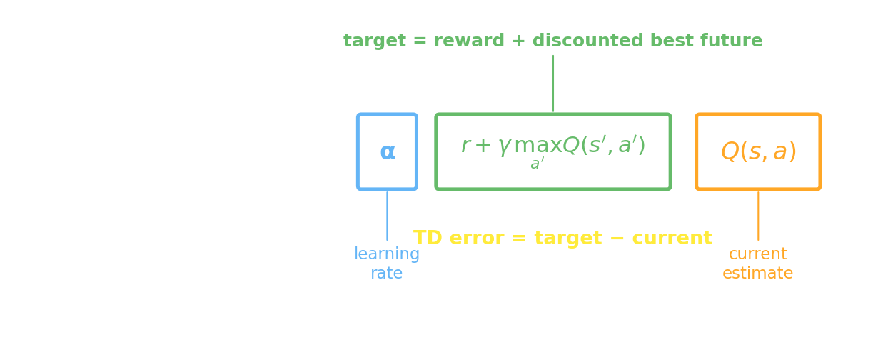
The nudge is the heart of it. Take action $a$ in state $s$; observe reward $r$ and next state $s'$. You now have a one-step glimpse of the truth: $r$ plus the discounted value of the best thing you can do from $s'$. Call that the target. The gap between the target and your current estimate is the temporal-difference (TD) error, and you move your estimate a fraction $\alpha$ of the way toward the target:
$$Q(s,a) \;\leftarrow\; Q(s,a) \;+\; \underbrace{\alpha}_{\text{learning rate}} \big[\, \underbrace{r + \gamma \max_{a'} Q(s',a')}_{\text{target}} \;-\; Q(s,a) \,\big].$$Two new symbols, each named as it lands: the learning rate $\alpha \in (0,1]$ controls how big each nudge is, and the bracketed quantity is the TD error — how surprised you were. If the target matches your estimate, the error is zero and nothing changes; if reality was better than expected, the error is positive and $Q$ rises. Learning is just repeatedly reducing surprise.
Notice what Q-learning doesn’t need: it never uses $T(s'\mid s,a)$. Where Chapter 21’s Bellman backup averaged over every next state with $\sum_{s'} T(s'\mid s,a)$, Q-learning uses the single $s'$ the world actually handed back — and over many visits those samples average out to the same expectation. That is what “model-free” means: you learn from the world’s responses, not from a map of the world. (The reward $r$ may now depend on the action too — the general $R(s,a)$ form Chapter 21 noted — since it’s whatever came back from the move you took.)
The TD error is a signal in your brain
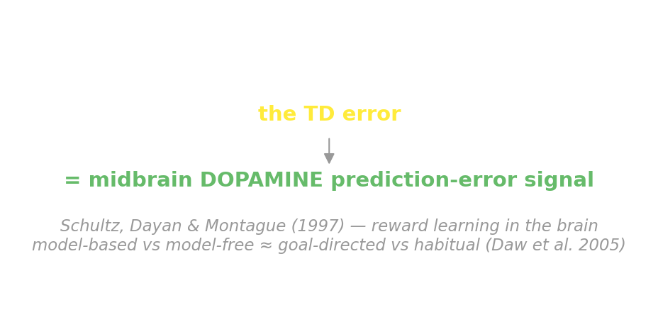
That bracketed surprise term — the TD error $r + \gamma\max_{a'}Q(s',a') - Q(s,a)$ — is not just a learning trick. It turns out to match, almost neuron for neuron, the moment-to-moment firing of midbrain dopamine neurons (Schultz, Dayan & Montague, 1997): they fire to reward prediction error — better or worse than expected — not to reward itself. A reward that is fully predicted produces no dopamine burst; a surprising one does; and an expected reward that fails to arrive produces a dip below baseline. That is exactly the TD error, with its sign. The little algebra you just wrote down is one of the best-supported theories of how brains learn to act — we’ll see its limits and the model-based counterpart later in the chapter.
GardenPath: a Grid to Learn
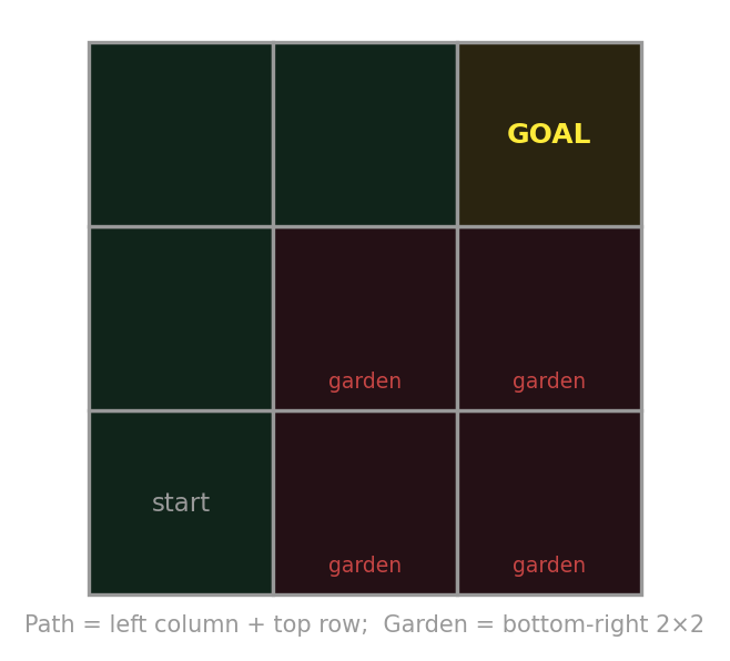
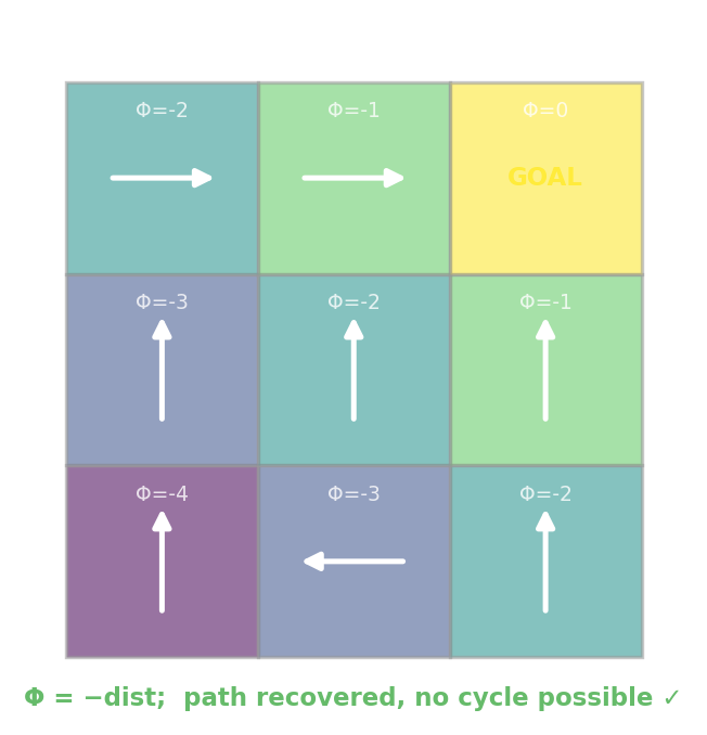
To watch Q-learning work, we need a world it can stumble around in. GardenPath (from Ho, Littman, Cushman & Austerweil, 2015) is a $3\times3$ grid. The agent starts bottom-left at $(1,1)$ and wants the top-right goal at $(3,3)$. The bottom-right $2\times2$ block is a garden to stay out of; the safe route — the path — is the left column then the top row, an L-shape:
The agent doesn’t know any of this. It only learns by moving (up/down/left/right) and collecting whatever reward each move returns. Here is the world and the Q-learning loop — $\varepsilon$-greedy exploration (act randomly a fraction $\varepsilon$ of the time, greedily otherwise), and the TD update on every step:
| |
Output:
Q-learning (rm) greedy path: (1,1) -> (2,1) -> (3,1) -> (3,2) -> (3,3) | reaches goal: TrueWith the natural reward-maximizing scheme — $+20$ for reaching the goal, $-10$ for stepping into the garden, $0$ otherwise — Q-learning, knowing nothing at the start, discovers the exact L-path from thousands of noisy trials. Step through it yourself in the widget: it single-steps the algorithm with a current-step indicator, shows the live $Q$-values as colored wedges and the greedy policy as arrows, and lets you switch the reward scheme — including a mode where you are the teacher.
(Try the “human — YOU are the teacher” mode: give the cat feedback move by move, then reveal whether your lessons actually reach the goal. It is harder than it looks — which is the whole point of the next section.)
Reward Shaping and Positive Cycles
Q-learning does exactly what you reward it for. That is its strength and its trap. The reward function is where you tell the agent what you want — and getting it subtly wrong produces an agent that’s perfectly optimal and completely useless.
Here is the trap, and it comes straight from how people naturally teach. When the agent does something good, you praise it ($+10$); when it backtracks along the path, you don’t punish it — you give faint praise ($+4$), because it’s still “on the right track.” That is the action-feedback scheme (af), and it encodes a real human bias: we reward effort and progress, not just outcomes. Watch what optimal behavior looks like under each scheme — solve all three exactly with value iteration (we know the rewards, so we can), and roll out the resulting greedy policy:
Output:
rm       : reaches the goal = True
af       : reaches the goal = False
potential: reaches the goal = True
The action-feedback agent never reaches the goal. It found a positive reward cycle: it paces back and forth forever, collecting praise, and never finishes. This is not a bug in Q-learning — it’s the optimal policy for the reward you gave. The agent is gaming you, exactly as you trained it to.
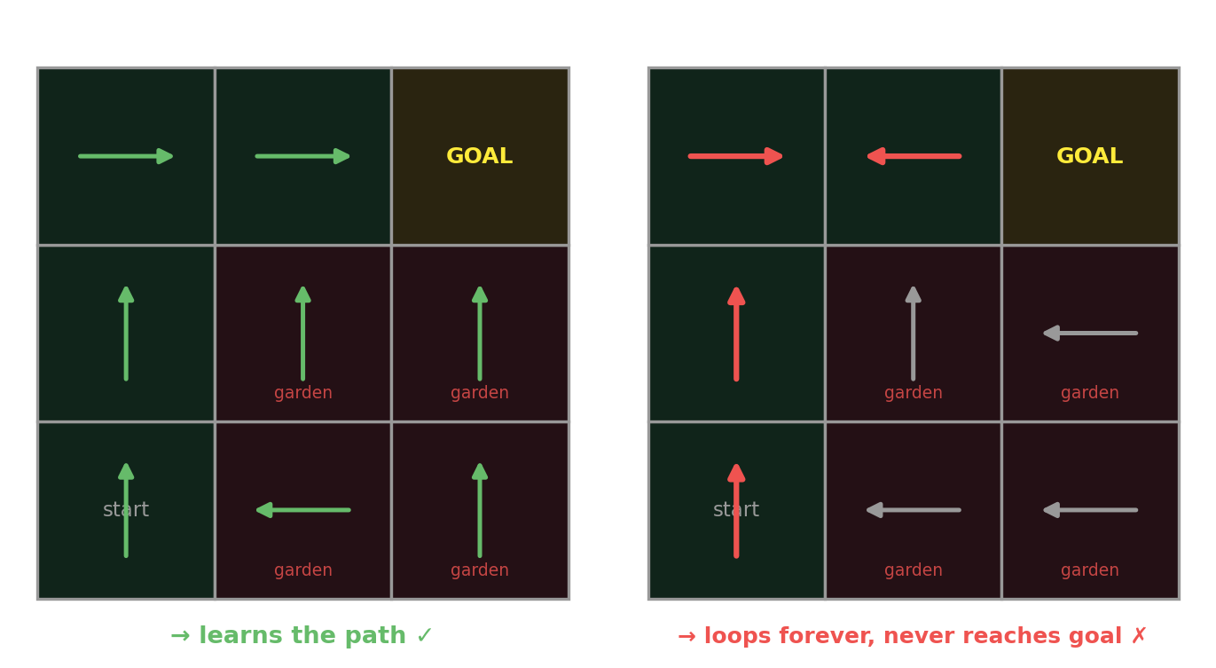
Why does looping win? Because the praise you can farm in a loop outweighs the one-time bonus for finishing. Pacing between two path cells collects $+10$ then $+4$, forever; finishing collects $+10$ then $+20$, once:
| |
Output:
value of looping forever  : 141.5
value of finishing the task: 29.0
A farmable loop worth $141.5$ buries the $29.0$ for finishing — so a perfectly rational agent loops. The fix is not to scold the agent but to shape the reward correctly. Potential-based shaping (Ng, Harada & Russell, 1999) adds a bonus built from a potential $\Phi(s)$ — here $\Phi = -(\text{Manhattan distance to goal})$ — in the precise form $F = \gamma\,\Phi(s') - \Phi(s)$. The magic is a telescoping identity: summed (with discounting) along any path $s_0, \dots, s_T$, these shaping rewards collapse to $\gamma^T\Phi(s_T) - \Phi(s_0)$ — a quantity that depends only on the endpoints, not the route. So shaping shifts every trajectory’s return by the same amount, leaving the optimal policy unchanged (Ng et al.’s policy-invariance theorem), while still nudging toward the goal on every step. See it directly — a path that loops for ages and a path that walks straight to the goal earn the same shaping total:
| |
Output:
discounted shaping, looping path  : 3.96
discounted shaping, finishing path: 4.00
both equal -Phi(start) = 4.00   -> the same constant, any route
The two routes earn the same shaping bonus (the tiny $3.96$-vs-$4.00$ gap is just $\gamma^T\Phi(s_T)$ for the looping path’s not-yet-at-goal endpoint, vanishing as the path lengthens), so the loop gains no farmable edge — and the potential row above confirms the optimal policy now reaches the goal. How you give feedback, not just how much, decides whether the agent does what you meant.
Simulation-Based RL: Planning with a Learned Model
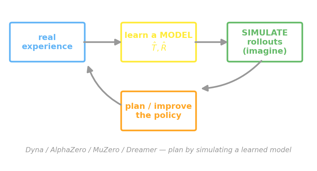
We have seen two extremes. Value iteration (Chapter 21) plans perfectly but needs the whole model. Q-learning learns from raw experience but needs many trials, because each real step teaches it only one thing. The frontier of RL lives in between: learn a model from experience, then plan by simulating with it. We’ll call this simulation-based RL (you may also hear “model-based RL”).
The simplest version is Dyna (Sutton, 1991): from experience, estimate a transition model $\hat T$ by counting where actions led, then run value iteration on $\hat T$ as if it were real. We leave GardenPath behind and return to the Chibany wellbeing MDP from Chapter 21 — we now want a model worth reconstructing. Recall its shape: three states — Junk ($R=+1$), Trying ($R=-2$), and Healthy ($R=+5$) — and two actions, Indulge (drift down) or Invest (climb up, but only by passing through the $-2$ Trying trough), at discount $\gamma = 0.9$:
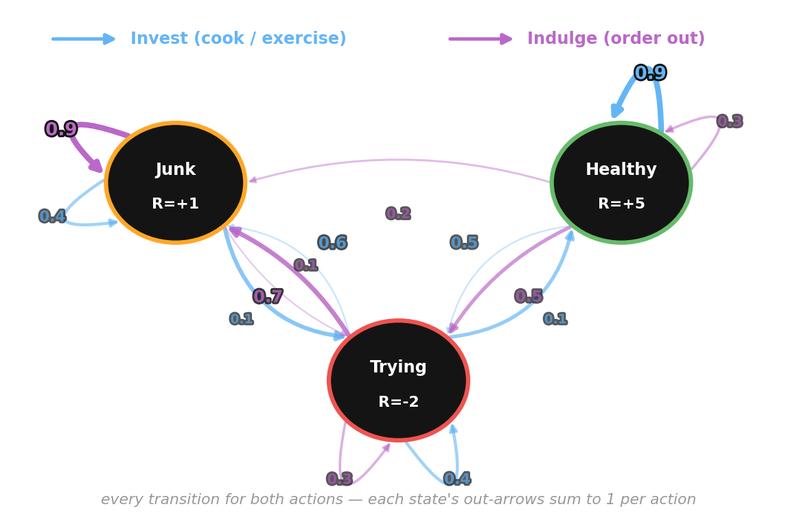
The agent never sees these probabilities — it just wanders randomly for a while, learns $\hat T$ by counting where its actions led, then plans on it. (Full Dyna interleaves the two, slipping a few imagined planning steps in after every real action; here we learn the model first and then plan, to keep the two stages clear.)
| |
Output:
Dyna (plan on the LEARNED model) policy: ['Invest', 'Invest', 'Invest']From nothing but random experience, the agent reconstructs enough of the world to recover the optimal Invest-everywhere policy — the same answer Chapter 21 computed from the true model. And this Dyna is GenJAX: every one of the 20 000 experience steps is a transition.simulate draw from the same @gen model as Chapter 21, and the whole random walk plus value iteration runs as a single JIT-compiled lax.scan — about 0.06 s.
This is a good moment to watch the two styles of learning side by side on the same Chibany MDP. Both agents see the identical stream of experience; the only difference is what they do with each step. Q-learning (model-free) makes one TD update per real step. Dyna (model-based) makes that same update plus a handful of planning backups from its learned model — replaying imagined experience to wring more out of every real step. Keep the exact answer from Chapter 21 in mind — value iteration gave $V^* = [25.6,\ 28.4,\ 39.8]$ with Invest optimal everywhere (the dashed targets). Watch both climb toward it; then drag Dyna’s planning steps to 0 and the two panels become identical — planning is the only difference:
With even a few planning steps, Dyna reaches the value-iteration answer in a fraction of the real experience Q-learning needs — the payoff of having a model to imagine with, the thread that runs from here to MCTS and AlphaZero.
Aside: Dyna point-estimates the model — the principled version is a POMDP
Dyna takes a shortcut worth naming. The empirical frequencies $\hat T = \text{counts} / \text{row totals}$ are the maximum-likelihood estimate of the transition matrix, and Dyna then plans as if that single estimate were exactly correct — a strategy called certainty equivalence: collapse the uncertainty to a point, then optimize. It works cleanly here only because we first gathered 20 000 steps under a random policy, so $\hat T$ is already sharp.
Keep the uncertainty instead and something elegant appears. Fold the unknown matrix into the state: let the true state be the pair $(s, \theta)$ where $\theta = T$ is hidden and static, and read every observed transition as an observation that sharpens a posterior over $\theta$ (a Dirichlet posterior — one per row, since each row’s counts are multinomial). That augmented problem is a genuine partially observable Markov decision process (POMDP) — an MDP whose true state you cannot see directly. In a POMDP the agent never observes the state $s$ itself; it receives only observations $o$ drawn from an observation model $O(o \mid s)$ that depend on the hidden state, so the best it can do is carry a belief — a probability distribution over which state it might be in — update that belief with each observation (by Bayes’ rule), and act on it. Our case is the structured one where the hidden part is the static parameters $\theta$ and the belief is the posterior over them — known as a Bayes-adaptive MDP. In it, “explore to pin down the dynamics” and “exploit what you already know” stop being separate phases and become a single optimization, because reducing uncertainty about $\theta$ now has value.
Solving that POMDP exactly is intractable, so the workhorse middle ground is posterior sampling (also called Thompson sampling): draw one plausible $T$ from the posterior, plan as if it were true, act, update, repeat — exploring each model in proportion to how plausible it still is. Dyna is the degenerate point-estimate corner of that same space. POMDPs are the subject of the next few chapters (still being written): partial observability is the rule, not the exception — a robot reading noisy sensors, a clinician inferring a disease from symptoms, a dialogue agent guessing a user’s intent all act without ever seeing the true state, and must plan over beliefs instead. The Bayes-adaptive view here is the bridge into that material: it shows that unknown parameters and unobserved state are the same machinery aimed at different parts of the state.
Telling Model-Free from Model-Based: The Two-Step Task
This chapter built both kinds of agent. Q-learning is model-free — it caches values from experience and never represents the world’s dynamics. Dyna is model-based — it holds a model and simulates it to plan, and the widget above let you watch the two learn side by side. That raises a question cognitive science cares about deeply: when a person (or a rat) learns a task, which kind of computation is the brain doing? You usually can’t tell from choices alone — given enough trials, both strategies solve the same task equally well. The trick is a task whose two systems are forced to predict different things. The framework it probes — a habitual model-free controller competing with a goal-directed model-based one — was introduced by Daw, Niv & Dayan (2005), who already used it to account for animal (rat) behavior; the human two-step task we walk through here, the first to dissociate the two systems in people, is Daw, Gershman, Seymour, Dayan & Dolan (2011), and it became one of the most influential paradigms in computational cognitive neuroscience.
The task. Recall from Chapter 1 that Chibany’s students bring them bentos — usually tonkatsu (Chibany’s favorite), sometimes a hamburger. The two-step task turns that into a daily choice with two stages. At stage 1 Chibany asks one of two students — Aki or Mei — for a bento. Which color box arrives is then only probabilistic: Aki usually brings the Red box (the common outcome, 70%) and Mei usually brings the Blue box (70% too); the other 30% of the time they swap (the rare outcome) and bring the other color. Inside, the box holds tonkatsu or a hamburger, and which color box tends to hold the tonkatsu drifts slowly day to day, so there is always something to keep learning. (Stage 1 = which friend to ask; the two color boxes are the two stage-2 states; tonkatsu is the reward.)
graph TD
    S1["Chibany asks: Aki or Mei?"]
    S1 -->|"Aki · 70% (usual)"| RED["Red box"]
    S1 -->|"Aki · 30% (swap)"| BLUE["Blue box"]
    S1 -->|"Mei · 70% (usual)"| BLUE
    S1 -->|"Mei · 30% (swap)"| RED
    RED --> R["tonkatsu or hamburger? (drifts slowly)"]
    BLUE --> R
    classDef node fill:none,stroke:#9bbcff,stroke-width:2px,color:#fff
    class S1,RED,BLUE,R node
    linkStyle default stroke:#9bbcff,stroke-width:2px,color:#fff
The whole game lives in that swap (the rare transition). Ask the simplest behavioral question: the next day, does Chibany ask the same friend (stay) or switch? The two systems answer from completely different information.
- Model-free asks only: did the friend I asked bring tonkatsu? A friend who brought tonkatsu gets reinforced, so Chibany is more likely to ask them again — full stop. It never consults which color box it came in. Prediction: a main effect of reward — tonkatsu → stay, hamburger → switch — with the swap making no difference.
- Model-based asks: which box held the tonkatsu, and which friend usually brings that box? Tonkatsu makes that box valuable, and Chibany then asks the friend who usually brings it. Here the swap bites. Say Chibany asked Aki, she swapped and brought the Blue box, and it held tonkatsu. The Blue box is now the prize — but the friend who usually brings Blue is Mei, not the Aki just asked. So model-based switches to Mei, even though asking Aki just got tonkatsu. Prediction: a reward × transition interaction (a crossover), not a plain reward effect.
That swap-with-tonkatsu case is the crux, and it is genuinely easy to tangle — so step through every combination yourself. Pick the friend, whether they brought their usual box or swapped, and what was inside, and watch what each mind concludes (the two verdicts agree on usual days and split on swap days):
We can also just simulate both agents. A model-free learner caches a value for each friend and nudges it toward the tonkatsu received; a model-based learner learns each color box’s value and combines them through the known 70/30 box habits to score the two friends. Run each for many days and tally how often Chibany asks the same friend, split by the previous day’s bento and whether the friend brought their usual box:
Output:
model-free    tonkatsu/usual 0.9  tonkatsu/swap 0.9   burger/usual 0.57  burger/swap 0.57
model-based   tonkatsu/usual 0.66  tonkatsu/swap 0.45   burger/usual 0.45  burger/swap 0.66
Those numbers are the signature. The model-free learner asks the same friend ~0.9 of the time after any tonkatsu and ~0.57 after any hamburger — flat across the swap. The model-based learner shows the crossover: ask again after a usual-day tonkatsu or a swap-day hamburger, switch after a swap-day tonkatsu or a usual-day hamburger. Plot the ask-again probability as two lines — one for tonkatsu days, one for hamburger days — across usual vs. swap, and model-free gives parallel lines (tonkatsu just shifts them together) while model-based gives crossing lines (the interaction). The widget runs the simulation live; slide the model-based weight $w$ from 0 to 1 to morph one into the other:
The result that made the task famous: real people show both — a reward main effect and an interaction, exactly the middle panel’s blend. That mixture is read as evidence that the brain runs the two systems in parallel and arbitrates between them — the habitual (model-free) and goal-directed (model-based) controllers of Daw et al. (2005). The plain model-free/model-based distinction this chapter drew in code turns out to be a measurable axis of human cognition.
Because the model-based score is a single number you can estimate per person, the task launched a large literature on individual differences: model-based control drops under stress and cognitive load, rises through childhood into adulthood, and — most influentially — tracks a transdiagnostic compulsivity dimension spanning OCD, addiction, and eating disorders (Gillan et al., 2016). It is one of the most-run paradigms in computational psychiatry.
A caution: the task is not a clean dissociation
For all its influence, the two-step task is an imperfect instrument, and it is worth knowing why. First, the standard version gives model-based control almost no reward advantage — a purely model-free agent earns nearly as much — so there is weak pressure to plan, the measure is noisy, and “low model-based control” can just mean “not worth the effort here” (Kool, Cushman & Gershman, 2016). Second, and more serious, the signature crossover is confounded: a sophisticated model-free learner whose state representation tracks the transition it just took can reproduce the very reward×transition interaction we called the model-based fingerprint, so the interaction is suggestive of planning, not proof of it (Akam, Costa & Dayan, 2015). Newer variants raise the model-based payoff and add controls, but the general lesson stands and is worth carrying out of this chapter: a behavioral signature is evidence about a computation, never the computation itself.
Planning by Search: MCTS
Back to planning with a model. Dyna reached the optimal policy by sweeping every state of its learned model — fine for Chibany’s three states, hopeless for a game with $10^{40}$ positions. The other great model-based method scales to exactly those worlds: Monte Carlo Tree Search (MCTS) samples the same kind of model, but estimates a state’s value by rollout — simulate many random-policy trajectories from a state and average their discounted returns. Written in GenJAX, that is one vmap-batched, compiled call over thousands of trajectories — which is where JAX earns its speed:
| |
Output:
GenJAX random-rollout value of Junk: 6.8(That low number is the random-rollout estimate — the same noisy default policy MCTS bootstraps from; the tree search is what lifts it toward the true value.)
Is there no efficient JAX/GenJAX MCTS? (Pedagogy vs. production)
There is, and it is worth being honest about. DeepMind’s mctx runs MCTS entirely in JAX — fully JIT-compiled and vmap-batched across many searches at once — and it is the search engine behind AlphaZero and MuZero. So why is the tree below written in plain NumPy? It is a readability choice, not a capability limit.
The catch is how you make a tree JAX-friendly. JAX cannot compile a tree that grows as Python dicts driven by a data-dependent while True loop — and the speed of the two cells above came entirely from batching fixed-size work (4000 rollouts through one kernel), which a grow-one-node-at-a-time loop can’t do. What mctx does instead is pre-allocate the whole tree as fixed-size arrays — visits[node, action], value_sums[…], and child/parent index arrays sized to the simulation budget — then run the four phases with lax.while_loop (descend and back up by walking the index arrays) and .at[idx].add(…) scatter updates. That compiles and runs fast on an accelerator, but it trades the readable dict-and-loop below for integer index-arithmetic that would bury the four-phase idea this section is teaching.
So the split is pedagogy vs. production, and the GenJAX piece carries over unchanged either way: the @gen transition model is the simulator you would hand to mctx’s recurrent function — only the bookkeeping around it changes. (For the record, the tempting shortcut — keeping the NumPy tree but swapping in a per-step transition.simulate call — is the worst of both worlds: measured here it runs over 20× slower, ≈33 s vs ≈1.4 s, because each call pays JAX dispatch overhead with nothing batched to amortize it. The NumPy np.random.choice(3, p=T[a, s]) below samples the identical distribution as categorical(jnp.log(T[a, s])) — same model, drawn the fast way for a loop that lives in host Python.) For readers who want to see it done properly, a runnable JAX MCTS — array-based tree, one compiled lax.scan, the GenJAX model doing every rollout step — is given in the optional “The Same Search, Compiled in JAX” section at the end of this part.
MCTS turns that rollout into a search: rather than commit to one fixed random policy, it simulates forward from where you are and steadily steers its rollouts toward the most promising moves, building a search tree with four repeated phases:
graph LR
    A["SELECT<br/>follow UCB down the tree"] --> B["EXPAND<br/>add a new node"]
    B --> C["SIMULATE<br/>random rollout to estimate value"]
    C --> D["BACKUP<br/>send the return up the path"]
    D --> A
    classDef node fill:none,stroke:#9bbcff,stroke-width:2px,color:#fff
    class A,B,C,D node
    linkStyle default stroke:#9bbcff,stroke-width:2px,color:#fff
The select phase chooses which action to follow by UCB — short for Upper Confidence Bound — a rule that balances taking the action that has looked best so far against trying one we have barely explored. For each action $a$ available at the current node it computes a score
$$\text{UCB}(a) \;=\; \underbrace{\frac{W_a}{N_a}}_{\text{exploit: average return}} \;+\; \underbrace{c\,\sqrt{\frac{\ln N_{\text{parent}}}{N_a}}}_{\text{explore: uncertainty bonus}},$$and picks the action with the highest score. Every symbol here is a running tally the tree keeps as it searches:
- $N_a$ — how many times action $a$ has been tried from this node so far.
- $W_a$ — the sum of the returns those $N_a$ tries earned, so $W_a / N_a$ is action $a$’s average return (the exploit term — favor what has paid off).
- $N_{\text{parent}} = \sum_{a'} N_{a'}$ — the node’s total visits, i.e. the sum of $N_{a'}$ over all of its actions.
- $c$ — the exploration constant (we use $c = 1.4$); a larger $c$ leans harder toward exploring.
The square-root term is the explore bonus: it is large when $N_a$ is small and shrinks as $a$ is tried more, so a rarely-taken action gets pulled up even when its current average is mediocre. (An untried action — $N_a = 0$ — has an infinite bonus, so MCTS tries each action once before it starts comparing averages.) UCB is the tree-search cousin of $\varepsilon$-greedy: instead of exploring at random, it explores where it is most uncertain.
A worked step makes the balance concrete. Suppose, partway through the search at the Junk node, we have tried Indulge $N_{\text{Indulge}} = 15$ times for a total return $W_{\text{Indulge}} = 210$ (average $14.0$), and Invest only $N_{\text{Invest}} = 2$ times for $W_{\text{Invest}} = 26$ (average $13.0$), so $N_{\text{parent}} = 15 + 2 = 17$. The two scores are
$$\text{Indulge}:\ \frac{210}{15} + 1.4\sqrt{\frac{\ln 17}{15}} = 14.0 + 0.61 = 14.61, \qquad \text{Invest}:\ \frac{26}{2} + 1.4\sqrt{\frac{\ln 17}{2}} = 13.0 + 1.67 = 14.67.$$Even though Indulge’s average ($14.0$) is the higher of the two, UCB selects Invest — because Invest has been tried so much less ($N=2$ vs $15$) that its uncertainty bonus ($1.67$) more than covers the $1.0$ gap in averages. That is the whole point: UCB keeps steering search toward actions it is unsure about, which is exactly how the under-tried Invest — the action that is actually optimal here — earns enough visits to reveal its true value. Each simulate step is then a rollout through the model — exactly the transition.simulate move from Chapter 21. Run MCTS from the Junk state of the Chibany MDP and it figures out the best action by simulating possible futures, no Bellman sweep required. (In the compact code below, select and expand share one loop iteration — the untried/UCB branch is both — and the four interactive widgets that follow pull the phases apart so you can watch each one.)
| |
Output:
MCTS from Junk picks: Invest (Q_Indulge=13.4, Q_Invest=17.0)MCTS recovers the optimal action — Invest — purely by simulating rollouts and keeping score, never once solving the Bellman equation. (One honest caveat: plain random rollouts make this a noisy estimator on a trap-then-reward MDP like Chibany’s — the optimal gap at Junk is thin, and random play rarely threads the $-2$ trough, so some seeds even prefer Indulge. That noise is exactly why AlphaZero replaces the random rollout with a learned value network.) The four phases are easiest to see one at a time. The first widget steps MCTS on this tiny Chibany tree, lighting up Select → Expand → Simulate → Backup so you can watch a single node’s estimate form:
The same four-phase loop scales to a real game. The second widget runs MCTS on tic-tac-toe — a deterministic, perfect-information game — growing a search tree move by move; then you can play against it:
This is the bridge to the most famous agents in AI. AlphaZero (Silver et al., 2018) is exactly this loop with the random rollout replaced by a learned value-and-policy network; MuZero (Schrittwieser et al., 2020) learns the model it searches in. They are MCTS, scaled.
Optional: The Same Search, Compiled in JAX
This part is for the curious — you can skip it without missing anything the rest of the course needs. The note above claimed an efficient JAX MCTS is real, just less readable than the NumPy one. Here is one, so the claim isn’t hand-waving. It plans on the same Chibany MDP, samples with the same @gen transition model, and runs the entire 4000-simulation search as a single JIT-compiled lax.scan — no Python loop over simulations, so none of the per-step dispatch cost that made the naive approach 20× slower.
The trick that makes it compile is to not grow a Python dict tree. Because the Chibany MDP has only three states, every statistic the search needs fits in two fixed $(3, 2)$ arrays — $N[s, a]$ (visit counts) and $W[s, a]$ (return sums), exactly the (state, action) keys the NumPy version used. Those two arrays are the carry of an outer lax.scan over simulations: each simulation reads them to choose actions by UCB and writes its results back with a scatter-add (.at[s, a].add(...)). Inside one simulation, an inner lax.scan walks horizon steps — descending by UCB while it can, then rolling out a random policy — with jnp.where standing in for every Python if so the whole thing is traceable:
Output:
JAX MCTS from Junk picks: Invest (Q_Indulge=5.6, Q_Invest=17.1)Same answer as the NumPy search — Invest — but the whole 4000-simulation run compiles to one kernel and finishes in under a fifth of a second. Two honest caveats keep it in perspective:
- It inherits the same noise. Random rollouts on this trap-then-reward MDP are nearly a coin-flip on the seed — some seeds lock onto Indulge instead (the NumPy search does too). That fragility is exactly why AlphaZero replaces the random rollout with a learned value network.
- It leans on the three-state shortcut. Keying statistics by
(state, action)only works because there are so few states. In a real game you can’t enumerate them, so a library like mctx pre-allocates the tree as node- and edge-indexed arrays and walks them with index arithmetic — more bookkeeping, but the same four phases, the same scan-and-scatter skeleton, and the same generative model doing the simulating.
Going further in the GenJAX ecosystem
The thread running through these three chapters — write the world as a generative model, then sample it to decide — is exactly what probabilistic programming is for. GenJAX is a general PPL, not an RL library, so the natural next step is the idea that planning is inference: a decision problem written as a generative model, solved with the same Monte-Carlo and SMC machinery you already know.
- Tutorial 2 — the deep dive on writing and querying generative functions in GenJAX (
simulate,generate,assess). - GenJAX & GenStudio — the GenJAX repo (modeling + programmable inference) and GenStudio (Python → interactive visualizations), from the MIT Probabilistic Computing Project; the broader Gen system underneath it.
- Planning as inference — Levine (2018), Reinforcement Learning and Control as Probabilistic Inference, and Moerland et al. (2023), A Unifying Framework for Reinforcement Learning and Planning — the formal version of “simulate to plan.”
- Coming later in the course (after the partial-observability and inverse-RL material): a dedicated chapter on world models (MuZero, Dreamer), deep RL at scale, and RLHF, where the agent must plan when it cannot even see the true state.
Where RL Is Now
The journey from a $3\times3$ grid to the frontier is one of scale, but every milestone is a piece you’ve now met:
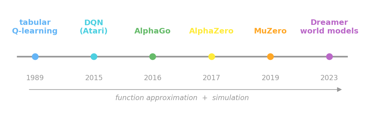
Tabular $Q$ became a neural network ($Q(s,a)$ predicted by a deep net — DQN (Mnih et al., 2015), which learned to play Atari from pixels); rollouts gained learned value and policy networks (AlphaGo, Silver et al., 2016; AlphaZero, Silver et al., 2018); and the model itself became learned (MuZero, Schrittwieser et al., 2020; Dreamer, Hafner et al., 2020). And the chapter’s central warning scales right along with it:
- Reward hacking is the positive cycle, at frontier scale. When a large language model is tuned with RL from human feedback (RLHF), the “reward” is a learned model of human approval — and agents reliably find ways to farm that approval without doing the underlying task, exactly as the action-feedback cat paced for praise. “Specify the reward you can measure, get the behavior you didn’t mean” is the same bug from the GardenPath, now a central problem in AI alignment (Weeks 11–13).
These ideas are not only engineering, either. The TD error you met at the start is a dopamine signal in the brain, and the model-free vs. model-based split is a measurable axis of cognition — the habitual-vs.-goal-directed systems the two-step task dissociates (Daw et al., 2005, 2011). Reinforcement learning is not just an engineering tool; it is one of our best theories of how brains learn to act.
What you can do now
You can run Q-learning — estimate action values $Q(s,a)$ from raw experience with the TD update, using a learning rate $\alpha$, $\varepsilon$-greedy exploration, and no model of the world — and you understand it learns the same optimal policy value iteration would, model-free. You know the central danger of reward design: a reward you can farm creates a positive cycle (the agent loops forever collecting praise), and that potential-based shaping is the principled fix because the shaping along any path collapses to a constant fixed by its endpoints, so no loop can farm it — the optimal policy is preserved. You can plan with a learned model — Dyna (count, then value-iterate) and MCTS (select → expand → simulate → backup) — which is simulation-based RL, the engine inside AlphaZero and MuZero. And you can see the two big through-lines: reward hacking is the positive cycle at scale, and the TD error is a dopamine signal in the brain.
This closes the agency arc that began in Chapter 20: from one decision, to planning a known world, to learning and acting in an unknown one. Next, the course turns to inverse RL — watching behavior and inferring the goals behind it.
Glossary: Q-learning, temporal-difference error, learning rate, ε-greedy, reward shaping, reward hacking, simulation-based RL, Monte Carlo Tree Search, UCB, certainty equivalence, Bayes-adaptive MDP, POMDP, two-step task.
Exercises
Try it yourself
- Watch it learn. In the
qlearncell, lowerepisodesto $200$ and rerun a few times with differentseeds. Does the greedy path always reach the goal? Now raise $\varepsilon$ to $0.5$ (much more exploration) — does it learn faster or slower, and why? - Break the reward yourself. In the human-teacher mode of the widget, try to teach the cat to reach the goal using only praise (👍) and neutral (➖) — no punishment. Can you avoid creating a positive cycle? Then explain, using the loop-vs-finish numbers, why “all carrots, no sticks” is so prone to looping.
- Sharpen MCTS. In the
mctscell, dropn_simto $100$ — does it still pick Invest reliably across seeds? Then raise the exploration constantcfrom its default of $1.4$ to $8.0$ and describe what happens to the gap betweenQ_InvestandQ_Indulge, and why over-exploring blurs the decision.
A companion notebook works through all of this interactively:
📓 Open in Colab: 22_q_learning.ipynb
References
- Akam, T., Costa, R., & Dayan, P. (2015). Simple plans or sophisticated habits? State, transition and learning interactions in the two-step task. PLOS Computational Biology, 11(12), e1004648. https://doi.org/10.1371/journal.pcbi.1004648
- Daw, N. D., Niv, Y., & Dayan, P. (2005). Uncertainty-based competition between prefrontal and dorsolateral striatal systems for behavioral control. Nature Neuroscience, 8(12), 1704–1711. https://doi.org/10.1038/nn1560
- Daw, N. D., Gershman, S. J., Seymour, B., Dayan, P., & Dolan, R. J. (2011). Model-based influences on humans’ choices and striatal prediction errors. Neuron, 69(6), 1204–1215. https://doi.org/10.1016/j.neuron.2011.02.027
- Gillan, C. M., Kosinski, M., Whelan, R., Phelps, E. A., & Daw, N. D. (2016). Characterizing a psychiatric symptom dimension related to deficits in goal-directed control. eLife, 5, e11305. https://doi.org/10.7554/eLife.11305
- Hafner, D., Lillicrap, T., Ba, J., & Norouzi, M. (2020). Dream to control: Learning behaviors by latent imagination. International Conference on Learning Representations (ICLR). https://arxiv.org/abs/1912.01603
- Ho, M. K., Littman, M. L., Cushman, F., & Austerweil, J. L. (2015). Teaching with rewards and punishments: Reinforcement or communication? Proceedings of the 37th Annual Conference of the Cognitive Science Society, 920–925.
- Kool, W., Cushman, F. A., & Gershman, S. J. (2016). When does model-based control pay off? PLOS Computational Biology, 12(8), e1005090. https://doi.org/10.1371/journal.pcbi.1005090
- Levine, S. (2018). Reinforcement learning and control as probabilistic inference: Tutorial and review. arXiv:1805.00909. https://arxiv.org/abs/1805.00909
- Mnih, V., Kavukcuoglu, K., Silver, D., et al. (2015). Human-level control through deep reinforcement learning. Nature, 518(7540), 529–533. https://doi.org/10.1038/nature14236
- Moerland, T. M., Broekens, J., Plaat, A., & Jonker, C. M. (2023). A unifying framework for reinforcement learning and planning. Frontiers in Artificial Intelligence, 6, 908353. https://doi.org/10.3389/frai.2023.908353
- Ng, A. Y., Harada, D., & Russell, S. (1999). Policy invariance under reward transformations: Theory and application to reward shaping. Proceedings of the 16th International Conference on Machine Learning (ICML), 278–287.
- Schrittwieser, J., Antonoglou, I., Hubert, T., et al. (2020). Mastering Atari, Go, chess and shogi by planning with a learned model. Nature, 588(7839), 604–609. https://doi.org/10.1038/s41586-020-03051-4
- Schultz, W., Dayan, P., & Montague, P. R. (1997). A neural substrate of prediction and reward. Science, 275(5306), 1593–1599. https://doi.org/10.1126/science.275.5306.1593
- Silver, D., Huang, A., Maddison, C. J., et al. (2016). Mastering the game of Go with deep neural networks and tree search. Nature, 529(7587), 484–489. https://doi.org/10.1038/nature16961
- Silver, D., Hubert, T., Schrittwieser, J., et al. (2018). A general reinforcement learning algorithm that masters chess, shogi, and Go through self-play. Science, 362(6419), 1140–1144. https://doi.org/10.1126/science.aar6404
- Sutton, R. S. (1991). Dyna, an integrated architecture for learning, planning, and reacting. ACM SIGART Bulletin, 2(4), 160–163. https://doi.org/10.1145/122344.122377
Special thanks to JPPCA for their generous support of this tutorial series.