Your First GenJAX Model

From Sets to Simulation

Remember Chibany’s daily meals? We listed out the outcome space $\Omega = \{HH, HT, TH, TT\}$ and counted possibilities.

Now we’ll teach a computer to generate those outcomes instead!

The Generative Process

Each day:

1. Lunch arrives — randomly H or T (equal probability)
2. Dinner arrives — randomly H or T (equal probability)
3. Record the day — the pair of meals

In GenJAX, we express this as a generative function.

Your First Generative Function

Here’s Chibany’s meals in GenJAX:

 1
 2
 3
 4
 5
 6
 7
 8
 9
10
11
12
13
14
15

import jax
from genjax import gen, flip

@gen
def chibany_day():
    """Generate one day of Chibany's meals."""

    # Lunch: flip a coin (0=Hamburger, 1=Tonkatsu)
    lunch_is_tonkatsu = flip(0.5) @ "lunch"

    # Dinner: flip another coin
    dinner_is_tonkatsu = flip(0.5) @ "dinner"

    # Return the pair
    return (lunch_is_tonkatsu, dinner_is_tonkatsu)

Breaking It Down

Line 1: @gen

• Tells GenJAX: “This is a generative function”
• GenJAX will track all random choices

Line 2-3: Function definition

• def chibany_day(): defines the function
• The docstring explains what it does

Line 6: First random choice

1

lunch_is_tonkatsu = flip(0.5) @ "lunch"

• flip(0.5) — Flip a fair coin (50% chance of 1, 50% chance of 0)
• @ "lunch" — Name this random choice “lunch”
• Store the result in lunch_is_tonkatsu

Line 9: Second random choice

1

dinner_is_tonkatsu = flip(0.5) @ "dinner"

• Another coin flip, named “dinner”

Line 12: Return value

1

return (lunch_is_tonkatsu, dinner_is_tonkatsu)

• Returns a tuple (pair) of the two values
• This is like one outcome from $\Omega$!

Running the Function

Generating One Day

1
2
3
4
5
6
7
8
9

# Create a random key (JAX requirement for randomness)
key = jax.random.key(42)

# Generate one day
trace = chibany_day.simulate(key, ())

# What happened?
meals = trace.get_retval()
print(f"Today's meals: {meals}")

Output (example):

Today's meals: (0, 1)

Today's meals: (Array(0, dtype=int32), Array(1, dtype=int32))

1
2
3

meals_simple = (int(meals[0]), int(meals[1]))
print(f"Today's meals: {meals_simple}")
# Output: (0, 1)

This means: Hamburger for lunch (0), Tonkatsu for dinner (1) — or in our notation: $HT$!

Accessing the Random Choices

1
2
3
4
5

# Get all the random choices made
choices = trace.get_choices()

print(f"Lunch was tonkatsu: {choices['lunch']}")
print(f"Dinner was tonkatsu: {choices['dinner']}")

Output (for the trace above):

Lunch was tonkatsu: 0
Dinner was tonkatsu: 1

Lunch was tonkatsu: 0
Dinner was tonkatsu: 1

Simulating Many Days

Now let’s generate 10,000 days!

 1
 2
 3
 4
 5
 6
 7
 8
 9
10
11
12
13
14
15
16

# Generate 10,000 random keys
import jax.numpy as jnp

keys = jax.random.split(key, 10000)

# Run the generative function for each key
def run_one_day(k):
    trace = chibany_day.simulate(k, ())
    return trace.get_retval()

# Use JAX's vmap for parallel execution
days_tuples = jax.vmap(run_one_day)(keys)

# Convert from tuples to a 2D array for easier analysis
# Each row is one day, columns are [lunch, dinner]
days = jnp.stack(days_tuples, axis=1)

Counting Outcomes

Now we have 10,000 days. Let’s count how many have at least one tonkatsu:

 1
 2
 3
 4
 5
 6
 7
 8
 9
10
11
12
13

import jax.numpy as jnp

# Check if either meal is tonkatsu (1)
has_tonkatsu = jnp.logical_or(days[:, 0], days[:, 1])

# Count how many days have tonkatsu
count_with_tonkatsu = jnp.sum(has_tonkatsu)

# Calculate probability
prob_tonkatsu = jnp.mean(has_tonkatsu)

print(f"Days with tonkatsu: {count_with_tonkatsu} out of 10000")
print(f"P(at least one tonkatsu) ≈ {prob_tonkatsu:.3f}")

Output (example):

Days with tonkatsu: 7489 out of 10000
P(at least one tonkatsu) ≈ 0.749

Remember from the probability tutorial: The exact answer is $3/4 = 0.75$!

With 10,000 simulations, we got very close: $0.749 \approx 0.75$

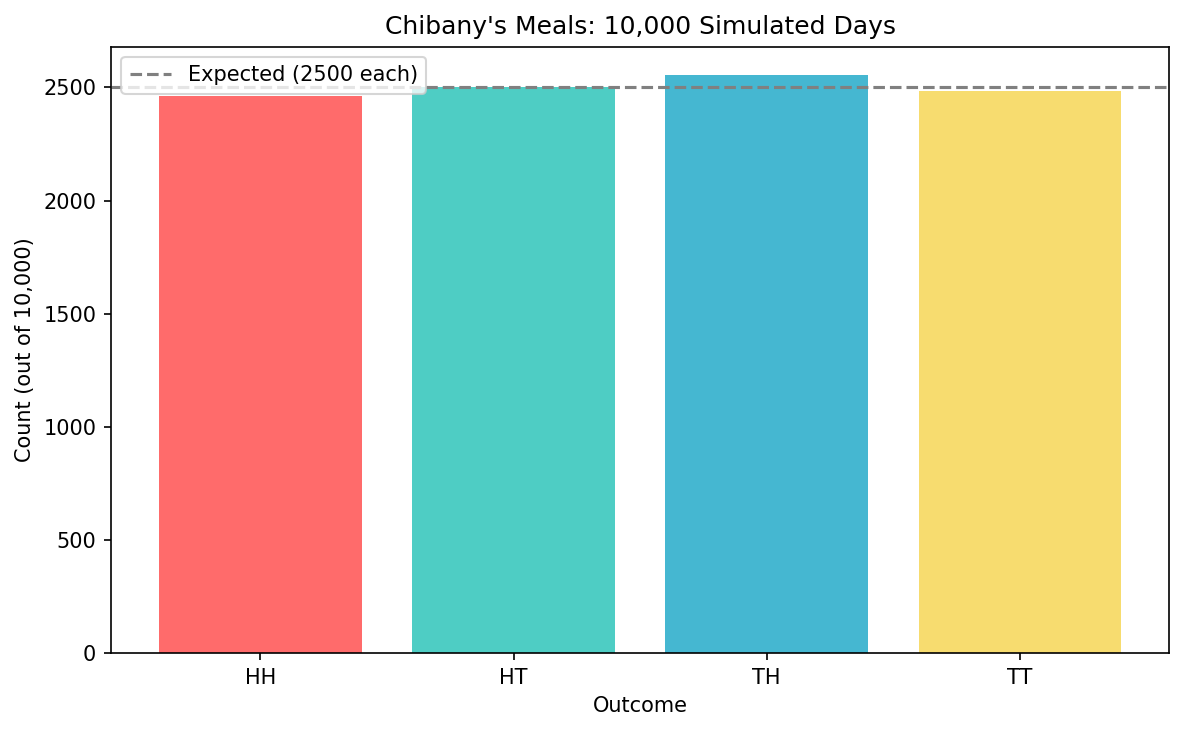
Visualizing the Results

Let’s make a bar chart showing all four outcomes:

 1
 2
 3
 4
 5
 6
 7
 8
 9
10
11
12
13
14
15
16
17
18
19
20
21
22

import matplotlib.pyplot as plt

# Count each outcome
import jax.numpy as jnp

HH = jnp.sum((days[:, 0] == 0) & (days[:, 1] == 0))
HT = jnp.sum((days[:, 0] == 0) & (days[:, 1] == 1))
TH = jnp.sum((days[:, 0] == 1) & (days[:, 1] == 0))
TT = jnp.sum((days[:, 0] == 1) & (days[:, 1] == 1))

# Create bar chart
outcomes = ['HH', 'HT', 'TH', 'TT']
counts = [HH, HT, TH, TT]

plt.figure(figsize=(8, 5))
plt.bar(outcomes, counts, color=['#ff6b6b', '#4ecdc4', '#45b7d1', '#f7dc6f'])
plt.xlabel('Outcome')
plt.ylabel('Count (out of 10,000)')
plt.title("Chibany's Meals: 10,000 Simulated Days")
plt.axhline(y=2500, color='gray', linestyle='--', label='Expected (2500 each)')
plt.legend()
plt.show()

What you’ll see: Four bars of roughly equal height (around 2500 each), matching our theoretical expectation of $1/4$ for each outcome!

Interactive Exploration

The companion notebook has interactive widgets so you can:

Slider 1: Probability of Tonkatsu for Lunch

• Move the slider from 0.0 to 1.0
• See how the distribution changes!

Slider 2: Probability of Tonkatsu for Dinner

• Make dinner independent from lunch
• Or make tonkatsu more/less likely at different meals

Slider 3: Number of Simulations

• Try 100, 1,000, 10,000, or even 100,000 simulations
• See how the estimate gets more accurate with more simulations

The chart updates automatically as you move the sliders!

Connection to Set-Based Probability

Let’s connect this back to what you learned:

Example:

Set-based:

• Event: “At least one tonkatsu” = $\{HT, TH, TT\}$
• Probability: $|\{HT, TH, TT\}| / |\{HH, HT, TH, TT\}| = 3/4$

GenJAX:

1
2
3
4

import jax.numpy as jnp

has_tonkatsu = (days[:, 0] == 1) | (days[:, 1] == 1)
prob = jnp.mean(has_tonkatsu)  # ≈ 0.75

It’s the same concept! Just computed instead of counted by hand.

Understanding Traces

When you run chibany_day.simulate(key, ()), GenJAX creates a trace that records:

1. Arguments — What inputs were provided (none in this case)
2. Random choices — All the random decisions made, with their names
3. Return value — The final result

1
2
3
4
5
6

trace = chibany_day.simulate(key, ())

# Access different parts
print(f"Return value: {trace.get_retval()}")
print(f"Choices: {trace.get_choices()}")
print(f"Log probability: {trace.get_score()}")

Output (example):

Return value: (Array(False, dtype=bool), Array(False, dtype=bool))
Choices: {'lunch': Array(False, dtype=bool), 'dinner': Array(False, dtype=bool)}
Log probability: -1.3862943611198906

What this means:

• Return value: The pair of meals (both False = both Hamburger = HH)
• Choices: A dictionary of all named random choices and their values
• Log probability: The log-likelihood of this particular outcome ($\log(0.5 \times 0.5) = \log(0.25) \approx -1.386$)

Exercises

Try these in the Colab notebook:

Exercise 1: Different Probabilities

Modify the code so:

• Lunch is 70% likely to be tonkatsu
• Dinner is 30% likely to be tonkatsu

Hint: Change the flip(0.5) values!

1
2
3
4
5

@gen
def chibany_day_weighted():
    lunch_is_tonkatsu = flip(0.7) @ "lunch"
    dinner_is_tonkatsu = flip(0.3) @ "dinner"
    return (lunch_is_tonkatsu, dinner_is_tonkatsu)

Exercise 2: Counting Tonkatsu

Write code to count how many tonkatsu Chibany gets across all simulated days (not just which days have tonkatsu, but the total count).

Hint: Add up days[:, 0] + days[:, 1]

1
2
3
4
5
6
7

import jax.numpy as jnp

total_tonkatsu = jnp.sum(days[:, 0]) + jnp.sum(days[:, 1])
avg_per_day = total_tonkatsu / len(days)

print(f"Total tonkatsu: {total_tonkatsu}")
print(f"Average per day: {avg_per_day:.2f}")

Exercise 3: Three Meals?

Extend the model to include breakfast! Now Chibany gets three meals per day.

1
2
3
4
5
6

@gen
def chibany_three_meals():
    breakfast_is_tonkatsu = flip(0.5) @ "breakfast"
    lunch_is_tonkatsu = flip(0.5) @ "lunch"
    dinner_is_tonkatsu = flip(0.5) @ "dinner"
    return (breakfast_is_tonkatsu, lunch_is_tonkatsu, dinner_is_tonkatsu)

What You’ve Learned

In this chapter, you:

✅ Wrote your first generative function

✅ Simulated thousands of random outcomes

✅ Calculated probabilities through counting

✅ Visualized distributions

✅ Understood the connection between sets and simulation

✅ Learned about traces and random choices

The key insight: Generative functions let computers do what you did by hand with sets — but now you can handle millions of possibilities!

Next Steps

Now that you can generate outcomes, the next question is:

What if I observe something? How do I update my beliefs?

That’s inference, and it’s where GenJAX really shines!