Conditioning and Inference
From Simulation to Inference
So far, we’ve used GenJAX to generate outcomes — simulating what could happen.
Now we’ll learn to infer — reasoning backwards from observations to causes.
This is the heart of probabilistic programming!

📓 Interactive Notebook Available
Prefer hands-on learning? This chapter has a companion Jupyter notebook - Open in Colab that walks through Bayesian inference interactively with working code, visualizations, and exercises. You can work through the notebook first, then return here for the detailed explanations, or use them side-by-side!
Recall: Conditional Probability
From the probability tutorial, remember conditional probability:
“Given that I observed $B$, what’s the probability of $A$?”
Written: $P(A \mid B)$
Meaning: Restrict the outcome space to only outcomes in $B$, then calculate the probability of $A$ within that restricted space.
Formula: $P(A \mid B) = \frac{P(A \cap B)}{P(B)} = \frac{|A \cap B|}{|B|}$
📘 Foundation Concept: Conditioning as Restriction
Recall from Tutorial 1, Chapter 4 that conditional probability means restricting the outcome space:
$$P(A \mid B) = \frac{|A \cap B|}{|B|}$$
The key idea: Cross out outcomes where $B$ didn’t happen, then calculate probabilities in what remains.
Tutorial 1 example: “At least one tonkatsu” given “first meal was tonkatsu”
- Original space: {HH, HT, TH, TT}
- Condition: First meal is T → Restrict to {TH, TT}
- Event: At least one T → In restricted space: {TH, TT}
- Probability: 2/2 = 1 (both remaining outcomes have tonkatsu!)
What GenJAX does:
- Tutorial 1: Manually cross out outcomes and count
- Tutorial 2: Code filters simulations or uses
ChoiceMapto restrict
The logic is identical — conditioning = restricting possibilities to match observations!
The Taxicab Problem: A Real Inference Challenge
Let’s apply these ideas to a real problem from the probability tutorial.
Scenario: Chibany witnesses a hit-and-run at night. They say the taxi was blue. But:
- 85% of taxis are green, 15% are blue
- Chibany identifies colors correctly 80% of the time
Question: What’s the probability it was actually a blue taxi?
Why This Is Surprising
Most people’s intuition says: “Chibany is 80% accurate, so probably 80% chance it’s blue.”
But the answer is only about 41%!
Why? Because most taxis are green. Even with 80% accuracy, there are more green taxis misidentified as blue than there are actual blue taxis correctly identified.
This is base rate neglect — ignoring how common something is in the population.
Let’s see how GenJAX helps us solve this!
The Generative Model
First, we express the taxicab scenario as a GenJAX generative function:
| |
What this encodes:
- Prior: Taxis are blue 15% of the time (base rate)
- Likelihood: How observation (“says blue”) depends on true color
- If blue: says “blue” 80% of the time (correct)
- If green: says “blue” 20% of the time (mistake)
- Complete model: Joint distribution over true color and observation
📘 Foundation Concept: Bayes’ Theorem in Code
Recall from Tutorial 1, Chapter 5 that Bayes’ Theorem updates beliefs with evidence:
$$P(H \mid E) = \frac{P(E \mid H) \cdot P(H)}{P(E)}$$
In the taxicab problem:
- Hypothesis (H): Taxi is blue
- Evidence (E): Chibany says “blue”
- Question: $P(\text{blue} \mid \text{says blue})$ = ?
Tutorial 1 approach (by hand):
- Calculate $P(\text{says blue} \mid \text{blue}) \cdot P(\text{blue}) = 0.80 \times 0.15 = 0.12$
- Calculate $P(\text{says blue} \mid \text{green}) \cdot P(\text{green}) = 0.20 \times 0.85 = 0.17$
- Calculate $P(\text{says blue}) = 0.12 + 0.17 = 0.29$
- Apply Bayes: $P(\text{blue} \mid \text{says blue}) = \frac{0.12}{0.29} \approx 0.41$
Tutorial 2 approach (GenJAX):
- Define the generative model (prior + likelihood)
- Specify observation (says blue)
- Let GenJAX compute the posterior automatically!
The structure is identical:
is_blue = flip(0.15)→ Prior: $P(\text{blue})$says_blue_prob = jnp.where(is_blue, accuracy, 1 - accuracy)→ Likelihood: $P(\text{says blue} \mid \text{blue})$- GenJAX conditioning → Computes posterior: $P(\text{blue} \mid \text{says blue})$
Key insight: GenJAX does all the Bayes’ Theorem algebra for you! You just write the generative story (prior + likelihood), and conditioning gives you the posterior.
Three Approaches to Inference
GenJAX provides three ways to compute conditional probabilities:
Approach 1: Filtering (Rejection Sampling)
Generate many traces, keep only those matching the observation.
Pseudocode:
1. Generate many traces
2. Keep only traces where observation is true
3. Among those, count how many satisfy the query
4. Calculate the ratio
This is Monte Carlo conditional probability — exactly what we did by hand with sets!
Approach 2: Conditioning with generate()
GenJAX has built-in support for specifying observations. We provide a choice map with the observed values, and GenJAX generates traces consistent with those observations.
Approach 3: Full Inference (Importance Sampling, MCMC)
More advanced methods (beyond this tutorial). These are more efficient when observations are rare.
This chapter focuses on Approach 1 and 2 — the most intuitive methods.
📐→💻 Math-to-Code Translation
How Bayesian inference translates to GenJAX:
| Math Concept | Mathematical Notation | GenJAX Code |
|---|---|---|
| Prior | $P(H)$ | flip(0.15) @ "is_blue" |
| Likelihood | $P(E \mid H)$ | jnp.where(is_blue, accuracy, 1-accuracy) |
| Evidence | $P(E)$ | GenJAX computes automatically |
| Posterior | $P(H \mid E) = \frac{P(E \mid H) P(H)}{P(E)}$ | Result of conditioning |
| Observation | $E$ = “says blue” | ChoiceMap.d({"says_blue": True}) |
| Inference Query | $P(\text{is_blue} \mid \text{says_blue})$ | mean(posterior_samples) |
Three equivalent inference approaches:
| Approach | Mathematical Idea | GenJAX Implementation |
|---|---|---|
| 1. Filtering | Sample from joint, keep only matching $E$ | Filter traces where says_blue == 1 |
| 2. generate() | Direct sampling from $P(H \mid E)$ | model.generate(key, observation, args) |
| 3. importance() | Weighted sampling | target.importance(key, n_particles) |
Key insights:
- Generative model = Prior + Likelihood — The @gen function encodes both
- Conditioning = Computing posterior — GenJAX does the Bayes’ theorem math
- All three methods compute the same thing — They just differ in efficiency
- Base rates matter! — Prior P(H) heavily influences posterior P(H|E)
Approach 1: Filtering (Rejection Sampling)
Let’s solve the taxicab problem by generating many scenarios and filtering to the observation.
Step 1: Generate Many Scenarios
| |
Step 2: Filter to Observation
Observation: Chibany says “blue”
| |
Output (example):
Scenarios where Chibany says blue: 29017 / 100000Why ~29%?
- $P(\text{says Blue}) = P(\text{Blue}) \cdot P(\text{says Blue} \mid \text{Blue}) + P(\text{Green}) \cdot P(\text{says Blue} \mid \text{Green})$
- $= 0.15 \times 0.80 + 0.85 \times 0.20 = 0.12 + 0.17 = 0.29$
Step 3: Count True Positives
Among scenarios where they say “blue”, how many are actually blue?
| |
Output (example):
Scenarios where taxi IS blue: 12038 / 29017Step 4: Calculate Posterior
| |
Output:
P(Blue | says Blue) ≈ 0.415Only 41.5%! Even though Chibany is 80% accurate, there’s less than 50% chance the taxi was actually blue!
The Base Rate Strikes!
Why so low?
Even though Chibany is 80% accurate, most taxis are green (85%). So even with his 20% error rate on green taxis, there are more green taxis misidentified as blue than there are actual blue taxis!
The numbers:
- Blue taxis correctly identified: $0.15 \times 0.80 = 0.12$ (12%)
- Green taxis incorrectly identified: $0.85 \times 0.20 = 0.17$ (17%)
More false positives than true positives!
This is why the posterior is only 41.5% ≈ 12/(12+17).
The Filtering Pattern
Conditional probability via filtering:
- Generate many traces
- Filter to observations (keep only matching traces)
- Count queries among filtered traces
- Divide to get conditional probability
This is rejection sampling — the simplest form of inference!
Approach 2: Using generate() with Observations
Now let’s use GenJAX’s built-in conditioning. This is usually more convenient!
Creating a Choice Map and Generating Conditional Traces
A choice map is a dictionary specifying values for named random choices. We use it to condition the model on observations:
| |
Output:
P(Blue | says Blue) ≈ 0.414Same answer! Both methods work — generate() is just more convenient.
⚠️ Critical: Always Use the Weights!
When using generate() with conditioning, you must use the importance weights returned!
Why? When GenJAX generates traces conditional on observations, different traces have different probabilities. The weight tells you how likely each trace is. Simply averaging without weights gives you the prior (what you believed before seeing the evidence), not the posterior (what you should believe after seeing the evidence).
Correct approach:
| |
Incorrect approach (gives wrong answer):
| |
This is the essence of importance sampling - a fundamental inference technique in probabilistic programming.
generate() vs simulate()
simulate(key, args):
- Generates a trace with all choices random
- No observations specified
- Returns just the trace
generate(key, observations, args):
- Generates a trace consistent with observations
- Specified choices take given values
- Unspecified choices are random
- Returns
(trace, weight)where weight = log probability of observations
When to use which:
- Forward simulation (no observations): Use
simulate() - Conditional sampling (some observations): Use
generate()
Theoretical Verification
Let’s verify our simulation against exact Bayes’ theorem calculation:
| |
Output:
=== Bayes' Theorem Calculation ===
P(Blue) = 0.15
P(says Blue | Blue) = 0.8
P(says Blue | Green) = 0.2
P(says Blue) = 0.29

P(Blue | says Blue) = 0.414
Perfect match! GenJAX simulation ≈ 0.415, Bayes’ theorem exact = 0.414
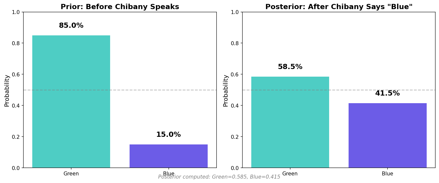
Visualizing Prior vs Posterior
Let’s visualize how evidence changes our beliefs:
| |
Key insight: Evidence increased our belief in blue from 15% to 41%, but still not even 50% because the base rate is so strong!
Exploring Base Rate Effects
Let’s see how changing the base rate affects the answer.
Scenario 1: Equal Taxis (50% blue, 50% green)
| |
Output:
If 50% blue: P(Blue | says Blue) = 0.800Now it’s 80%! When base rates are equal, accuracy dominates.
Scenario 2: Mostly Blue (85% blue, 15% green)
| |
Output:
If 85% blue: P(Blue | says Blue) = 0.971Now it’s 97%! When most taxis are blue, seeing “blue” is strong evidence.
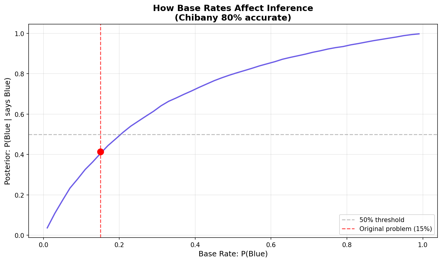
Visualizing the Effect
| |
The graph shows a sigmoidal (S-shaped) curve:
- Low base rates (e.g., 1%): Even with a positive witness, posterior stays low (~4%)
- Medium base rates (e.g., 50%): Steep rise - evidence has maximum impact (~80%)
- High base rates (e.g., 99%): Posterior approaches certainty (~99.7%)
The curve shows: Even with 80% accuracy, the posterior depends heavily on the base rate!
The Lesson
Base rates matter enormously in real-world inference!
Medical tests, fraud detection, witness testimony — all require considering:
- How accurate is the test/witness? (likelihood)
- How common is the condition/crime? (prior/base rate)
Ignoring base rates leads to wrong conclusions.
This is called base rate neglect — a common cognitive bias.
Key Concepts
Prior Distribution
What we believe before seeing data.
- Generated by
simulate()(no observations) - Represents our initial uncertainty
Posterior Distribution
What we believe after seeing data.
- Generated by
generate()with observations - Represents updated beliefs incorporating evidence
Bayes’ Theorem in Action
GenJAX automatically handles the math:
$$P(\text{hypothesis} \mid \text{data}) = \frac{P(\text{data} \mid \text{hypothesis}) \cdot P(\text{hypothesis})}{P(\text{data})}$$
You just:
- Define the generative model (encodes $P(\text{data} \mid \text{hypothesis})$ and $P(\text{hypothesis})$)
- Specify observations (the data)
- Generate conditional traces (GenJAX computes the posterior)
No manual Bayes’ rule calculation needed!
The Power of Generative Models
When you write a generative function, you’re specifying:
- Prior: The distribution of random choices before observations
- Likelihood: How observations depend on hidden variables
- Joint distribution: The complete probabilistic model
GenJAX handles the inference automatically!
Complete Example Code
Here’s everything together for easy copying:
| |
Interactive Exploration
📓 Interactive Notebook: Bayesian Learning
Want to explore Bayesian learning in depth with interactive examples? Check out the Bayesian Learning notebook - Open in Colab which covers:
- The complete taxicab problem with visualizations
- Sequential Bayesian updating with multiple observations
- Interactive sliders to explore different base rates and accuracies
- How base rates affect posterior beliefs
This notebook lets you experiment with the concepts you just learned!
Exercises
Exercise 1: Higher Accuracy
What if Chibany were 95% accurate instead of 80%?
Task: Modify the code to use accuracy=0.95 and calculate the posterior.
Exercise 2: Opposite Observation
What if Chibany said “green” instead of “blue”?
Task: Calculate $P(\text{Blue} \mid \text{says Green})$
Exercise 3: Two Witnesses
What if two independent witnesses both say “blue”?
Task: Extend the model to include two witnesses, both 80% accurate. Calculate the posterior.
What You’ve Learned
In this chapter, you learned:
✅ Conditional probability — restriction to observations
✅ Filtering approach — rejection sampling for inference
✅ generate() function — conditioning with choice maps
✅ Prior vs Posterior — beliefs before and after data
✅ Bayes’ theorem in action — automatic Bayesian update
✅ Base rate effects — why priors matter enormously
✅ Real inference problems — the taxicab scenario
The key insight: Probabilistic programming lets you encode assumptions (generative model) and ask questions (conditioning) without manual Bayes’ rule calculations!
Why This Matters
Real-world applications:
- Medical diagnosis: Test accuracy + disease prevalence → probability of disease
- Fraud detection: Transaction patterns + fraud base rate → probability of fraud
- Spam filtering: Email features + spam base rate → probability of spam
- Criminal justice: Witness accuracy + crime base rate → probability of guilt
All follow the same pattern:
- Define generative model (how data arises)
- Observe data
- Infer hidden causes
GenJAX makes this systematic and scalable.
Next Steps
You now know:
- How to build generative models
- How to perform inference with observations
- How to interpret posterior probabilities
- Why base rates matter
Next up: Chapter 6 shows you how to build your own models from scratch!
| ← Previous: Understanding Traces | Next: Building Your Own Models → |
|---|