Chibany's Mystery Bentos

The Weight of the Matter

It’s a new semester at the university, and Chibany’s students have been bringing them bentos again. But this time, something is different.

Last semester, the bento boxes were transparent. So Chibany could see whether there was tonkatsu or hamburger inside. But this semester, the bento boxes are opaque. Thus, Chibany can’t see what is inside when they receive the bento. They want to know IMMEDIATELY what the meal is, but it would be extremely rude to open the bento box as the students are watching. Thankfully, Chibany is curious, and they’re a probabilist.

So they hatch a plan: weigh the bentos.

Tonkatsu bentos are hearty and heavy. Hamburger bentos are lighter. If they record the weights, maybe they can figure out what they’ve been receiving, and even predict what’s coming next.

Overheard Conversation

One afternoon, while Chibany is napping, they overhear two students chatting nearby:

Student 1: “I’ve been bringing Chibany tonkatsu most days. It’s their favorite!” Student 2: “Me too! Though sometimes I bring hamburger when the cafeteria runs out of tonkatsu.” Student 1: “Yeah, I’d say I bring tonkatsu like… seven times out of ten?” Student 2: “Same! About 70% tonkatsu, 30% hamburger.”

Chibany smiles. So there is a pattern! But they decide to continue their experiment anyway. Can they discover this 70-30 split just from weighing the bentos?

Week One: Something Strange

Chibany weighs their first week of bentos and records the measurements:

Monday:    520g
Tuesday:   348g
Wednesday: 505g
Thursday:  362g
Friday:    488g

They calculate the average: 441 grams.

“Hmm,” they think, “that’s odd. Last semester, tonkatsu bentos weighed about 500g and hamburger bentos weighed about 350g. But 441g is right in the middle! Am I getting medium-sized bentos?”

They weigh more bentos over the next few weeks:

Week 2: 355g, 510g, 492g, 345g, 515g
Week 3: 498g, 358g, 505g, 362g, 490g
Week 4: 352g, 488g, 508g, 355g, 495g

After a month, they have 20 measurements. The average is still around 445g.

But something doesn’t add up…

The Paradox Revealed

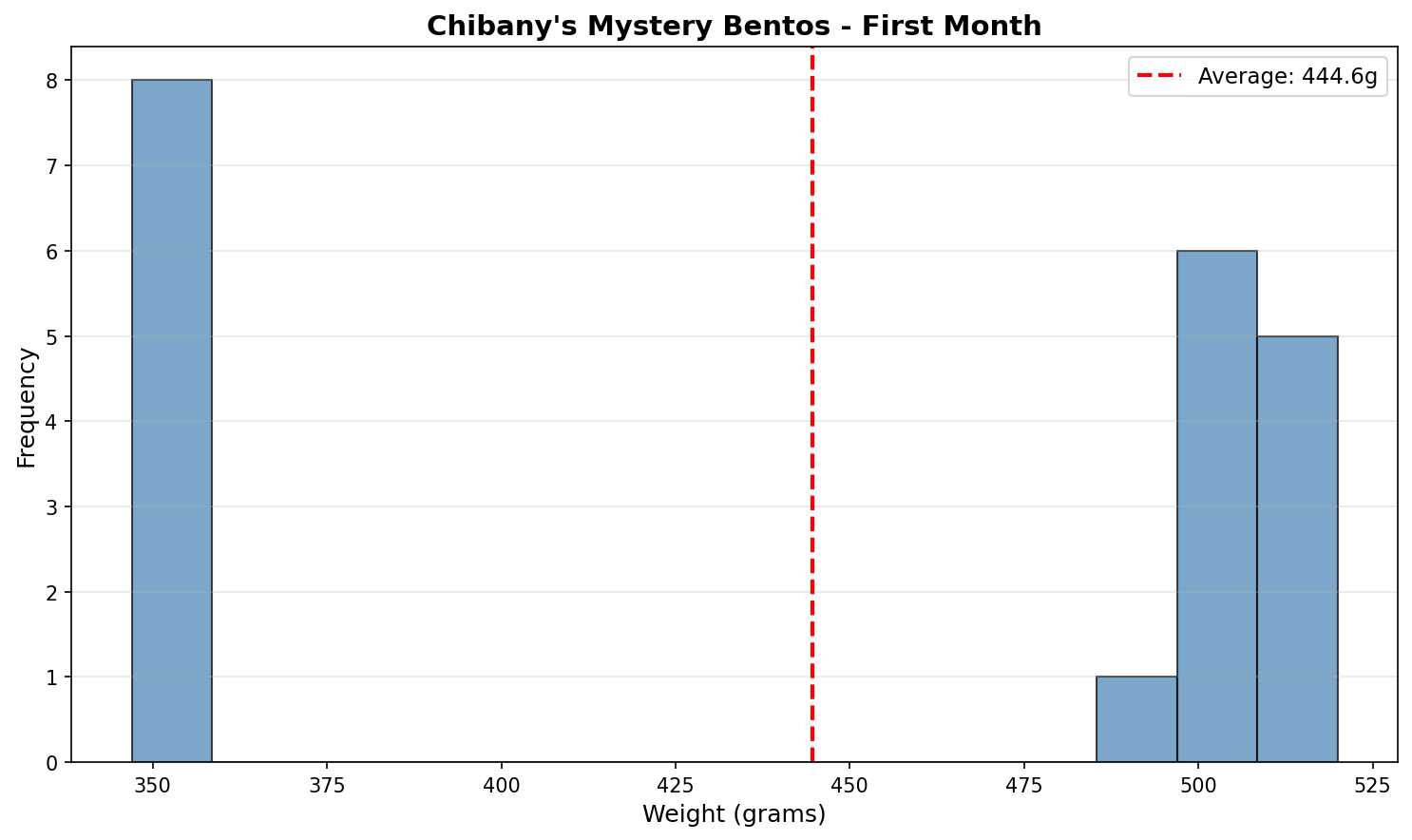
Chibany plots their measurements on a histogram:

 1
 2
 3
 4
 5
 6
 7
 8
 9
10
11
12
13
14

import numpy as np

# Chibany's actual measurements (grams)
weights = np.array([
    520, 348, 505, 362, 488,  # Week 1
    355, 510, 492, 345, 515,  # Week 2
    498, 358, 505, 362, 490,  # Week 3
    352, 488, 508, 355, 495   # Week 4
])

print(f"Average weight: {weights.mean():.1f}g")
print(f"Weights near 350g: {np.sum((weights >= 340) & (weights <= 370))}")
print(f"Weights near 500g: {np.sum((weights >= 480) & (weights <= 520))}")
print(f"Weights near 445g: {np.sum((weights >= 435) & (weights <= 455))}")

 1
 2
 3
 4
 5
 6
 7
 8
 9
10
11
12
13
14
15

import matplotlib.pyplot as plt

# Create histogram
plt.figure(figsize=(10, 6))
plt.hist(weights, bins=15, edgecolor='black', alpha=0.7, color='steelblue')
plt.axvline(weights.mean(), color='red', linestyle='--', linewidth=2,
            label=f'Average: {weights.mean():.1f}g')
plt.xlabel('Weight (grams)', fontsize=12)
plt.ylabel('Frequency', fontsize=12)
plt.title("Chibany's Mystery Bentos - First Month", fontsize=14, fontweight='bold')
plt.legend(fontsize=11)
plt.grid(axis='y', alpha=0.3)
plt.tight_layout()
plt.savefig('mystery_bentos_histogram.png', dpi=150, bbox_inches='tight')
plt.show()

Output:

Average weight: 445.4g
Weights near 350g: 6
Weights near 500g: 14
Weights near 445g: 0

They stare at the plot. Something is very wrong.

Most weights cluster around 350g (hamburger range). Most others cluster around 500g (tonkatsu range). But ZERO measurements are near 445g (the average)!

The Resolution: Expected Value

Chibany has an insight. They’re not receiving “medium bentos.” They’re receiving a mixture of heavy tonkatsu bentos and light hamburger bentos!

Looking at the data more carefully:

• About 14 out of 20 measurements are near 500g (tonkatsu)
• About 6 out of 20 measurements are near 350g (hamburger)

That’s roughly:

• 70% tonkatsu (θ = 0.7), just like the students said!
• 30% hamburger (θ = 0.3)

Now the 445g average makes sense! It’s not that individual bentos weigh 445g. It’s that the long-run average of the mixture is:

$$\text{Average weight} = (0.7 \times 500\text{g}) + (0.3 \times 350\text{g}) = 350 + 105 = 455\text{g}$$

Their observed average of 445g is close to the theoretical 455g. The difference is just random variation from a small sample.

This is called the expected value, written $E[X]$.

What Is Expected Value?

In plain English: Expected value is what you’d get “on average” if you repeated something many, many times.

For Chibany’s bentos:

• 70% of days he gets tonkatsu (500g)
• 30% of days he gets hamburger (350g)
• On average over many days, his bento weighs: (0.7 × 500) + (0.3 × 350) = 455g

The mathematical definition: Expected value is the weighted average of all possible outcomes, where the weights are the probabilities.

For a discrete random variable $X$ that can take values $x_1, x_2, \ldots, x_n$ with probabilities $p_1, p_2, \ldots, p_n$:

$$E[X] = \sum_{i=1}^{n} p_i \cdot x_i$$

Breaking this down:

• $p_i$ = probability of outcome $i$
• $x_i$ = value of outcome $i$
• $\sum$ = “add them all up”

In Chibany’s case:

• $X$ = weight of a bento
• $x_1 = 500$ (tonkatsu weight) with probability $p_1 = 0.7$
• $x_2 = 350$ (hamburger weight) with probability $p_2 = 0.3$

Therefore: $$E[X] = 0.7 \times 500 + 0.3 \times 350 = 455\text{g}$$

Three Key Insights

1. Expected value ≠ “expected” in the everyday sense

You shouldn’t “expect” any single bento to weigh exactly 455g. In fact, almost no bento weighs 455g! The term “expected value” is a bit misleading. It really means “long-run average.”

2. Expected value is the center of mass

Imagine the histogram balanced on a seesaw. Where would you put the fulcrum so it balances? At the expected value! It’s the distribution’s “center of gravity.”

3. Expected value hides the structure

Knowing $E[X] = 455\text{g}$ doesn’t tell you there are two distinct types of bentos. You lose the bimodal structure (two peaks). That’s why we’ll need more tools (like variance and mixture models) to fully understand distributions.

Common Misconceptions About Expected Value

Visualizing Expected Value as Balance Point

Let’s see why E[X] is called the “balance point” by trying different fulcrum positions:

  1
  2
  3
  4
  5
  6
  7
  8
  9
 10
 11
 12
 13
 14
 15
 16
 17
 18
 19
 20
 21
 22
 23
 24
 25
 26
 27
 28
 29
 30
 31
 32
 33
 34
 35
 36
 37
 38
 39
 40
 41
 42
 43
 44
 45
 46
 47
 48
 49
 50
 51
 52
 53
 54
 55
 56
 57
 58
 59
 60
 61
 62
 63
 64
 65
 66
 67
 68
 69
 70
 71
 72
 73
 74
 75
 76
 77
 78
 79
 80
 81
 82
 83
 84
 85
 86
 87
 88
 89
 90
 91
 92
 93
 94
 95
 96
 97
 98
 99
100
101
102
103
104
105
106
107
108
109
110
111
112
113
114
115
116
117
118
119
120
121
122
123
124
125
126
127
128
129
130
131
132

import numpy as np
import matplotlib.pyplot as plt
from matplotlib.patches import Circle, Polygon

def draw_seesaw_panel(ax, fulcrum_position, title, show_calculation=True):
    """Draw a single seesaw panel with given fulcrum position"""

    # Bento positions and masses
    pos_hamburger = 350
    pos_tonkatsu = 500
    mass_hamburger = 0.3
    mass_tonkatsu = 0.7

    # Calculate distances from fulcrum
    dist_hamburger = abs(pos_hamburger - fulcrum_position)
    dist_tonkatsu = abs(pos_tonkatsu - fulcrum_position)

    # Calculate torques
    torque_left = mass_hamburger * dist_hamburger if pos_hamburger < fulcrum_position else 0
    torque_right = mass_tonkatsu * dist_tonkatsu if pos_tonkatsu > fulcrum_position else 0

    if pos_hamburger > fulcrum_position:
        torque_right += mass_hamburger * dist_hamburger
    if pos_tonkatsu < fulcrum_position:
        torque_left += mass_tonkatsu * dist_tonkatsu

    net_torque = torque_right - torque_left

    # Calculate rotation angle (exaggerated for visibility)
    max_angle = 25  # degrees
    rotation_angle = np.clip(net_torque * max_angle / 50, -max_angle, max_angle)

    # Draw seesaw
    seesaw_length = 200
    seesaw_left = fulcrum_position - seesaw_length / 2
    seesaw_right = fulcrum_position + seesaw_length / 2

    # Apply rotation
    angle_rad = np.radians(rotation_angle)
    left_y = -seesaw_length / 2 * np.sin(angle_rad)
    right_y = seesaw_length / 2 * np.sin(angle_rad)

    # Draw the seesaw plank
    ax.plot([seesaw_left, seesaw_right], [left_y, right_y],
            'k-', linewidth=6, solid_capstyle='round', zorder=2)

    # Draw fulcrum (triangle)
    triangle_size = 15
    triangle = Polygon([
        [fulcrum_position - triangle_size/2, -triangle_size],
        [fulcrum_position + triangle_size/2, -triangle_size],
        [fulcrum_position, 0]
    ], facecolor='red', edgecolor='darkred', linewidth=2, zorder=3)
    ax.add_patch(triangle)

    # Draw bento masses (circles positioned on seesaw)
    # Calculate actual positions on rotated seesaw
    hamburger_offset = pos_hamburger - fulcrum_position
    tonkatsu_offset = pos_tonkatsu - fulcrum_position

    hamburger_y = hamburger_offset * np.sin(angle_rad)
    tonkatsu_y = tonkatsu_offset * np.sin(angle_rad)

    # Hamburger bento
    circle_hamburger = Circle((pos_hamburger, hamburger_y + 8),
                             radius=8, facecolor='orange',
                             edgecolor='darkorange', linewidth=2, zorder=4)
    ax.add_patch(circle_hamburger)
    ax.text(pos_hamburger, hamburger_y + 25, '30%\n(350g)',
           ha='center', va='center', fontsize=10, fontweight='bold')

    # Tonkatsu bento (larger circle to show 70%)
    circle_tonkatsu = Circle((pos_tonkatsu, tonkatsu_y + 8),
                            radius=12, facecolor='brown',
                            edgecolor='saddlebrown', linewidth=2, zorder=4)
    ax.add_patch(circle_tonkatsu)
    ax.text(pos_tonkatsu, tonkatsu_y + 30, '70%\n(500g)',
           ha='center', va='center', fontsize=10, fontweight='bold')

    # Mark fulcrum position
    ax.axvline(fulcrum_position, color='red', linestyle=':', alpha=0.5, zorder=1)
    ax.text(fulcrum_position, -40, f'Fulcrum\n{fulcrum_position}g',
           ha='center', va='top', fontsize=9, color='red', fontweight='bold')

    # Show calculation if requested
    if show_calculation:
        calc_text = f"Left torque: {torque_left:.1f}\nRight torque: {torque_right:.1f}"
        ax.text(0.05, 0.95, calc_text, transform=ax.transAxes,
               fontsize=9, va='top', bbox=dict(boxstyle='round',
               facecolor='wheat', alpha=0.8))

    # Determine balance state
    if abs(rotation_angle) < 1:
        balance_state = "⚖️ BALANCED!"
        balance_color = 'green'
    elif rotation_angle > 0:
        balance_state = "↻ TIPS RIGHT"
        balance_color = 'red'
    else:
        balance_state = "↺ TIPS LEFT"
        balance_color = 'blue'

    # Title with balance state
    ax.text(0.5, 0.98, title, transform=ax.transAxes,
           ha='center', va='top', fontsize=12, fontweight='bold')
    ax.text(0.5, 0.88, balance_state, transform=ax.transAxes,
           ha='center', va='top', fontsize=14, fontweight='bold',
           color=balance_color)

    # Clean up axes
    ax.set_xlim(320, 530)
    ax.set_ylim(-50, 50)
    ax.set_aspect('equal')
    ax.axis('off')

# Create figure with 3 panels
fig, (ax1, ax2, ax3) = plt.subplots(1, 3, figsize=(16, 5))

# Panel 1: Fulcrum too far left (tips right)
draw_seesaw_panel(ax1, 400, "Fulcrum at 400g")

# Panel 2: Fulcrum too far right (tips left)
draw_seesaw_panel(ax2, 480, "Fulcrum at 480g")

# Panel 3: Fulcrum at E[X] (balanced!)
draw_seesaw_panel(ax3, 455, "Fulcrum at E[X] = 455g")

plt.suptitle("Why E[X] is the Balance Point",
            fontsize=16, fontweight='bold', y=1.02)
plt.tight_layout()
plt.savefig('seesaw_balance_point.png', dpi=150, bbox_inches='tight')
plt.show()

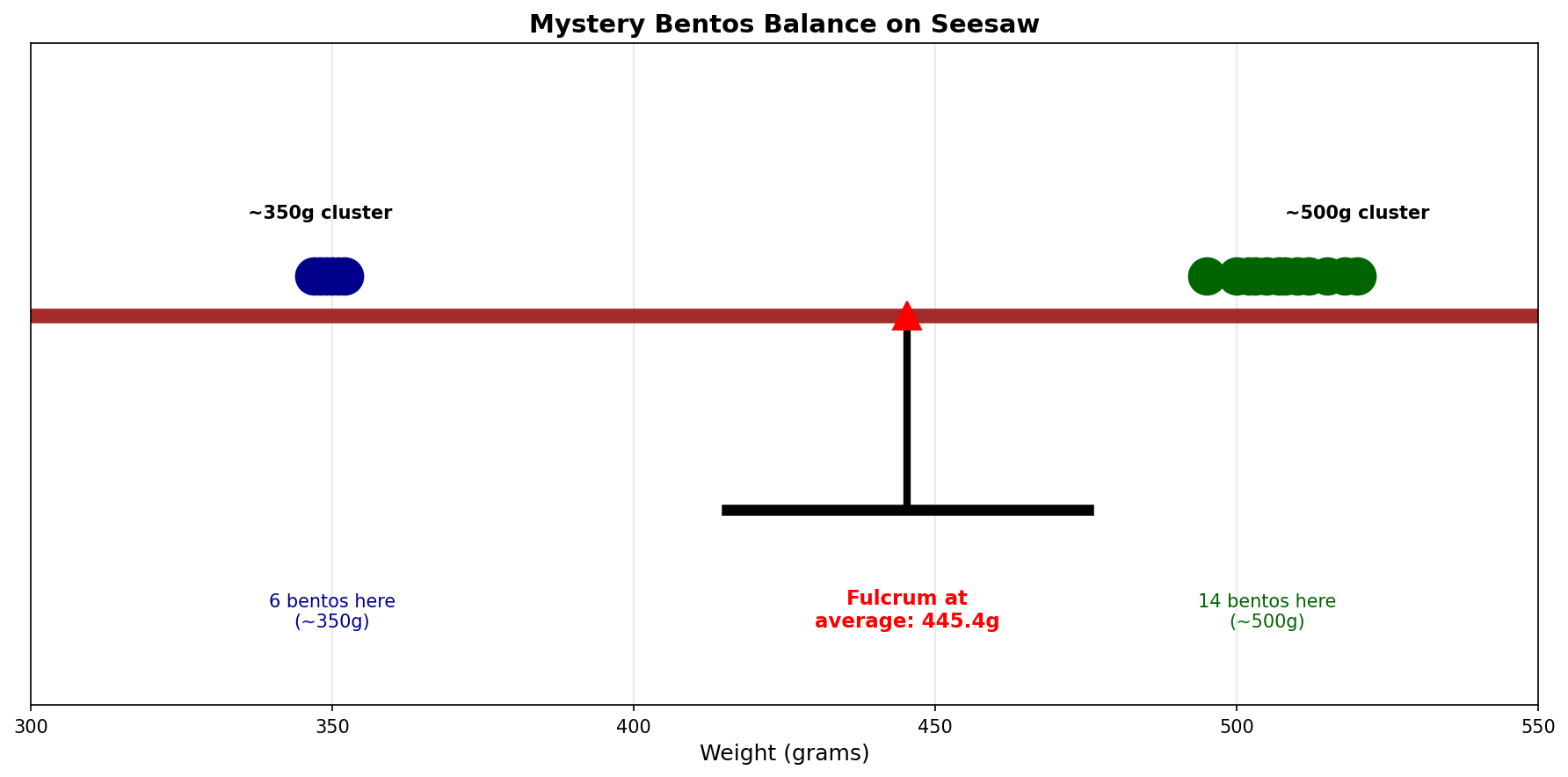
The expected value E[X] = 455g is the unique position where the distribution balances.

Think of it like a seesaw at a playground:

• When the fulcrum is at 400g, the heavy tonkatsu side (70% probability at 500g) outweighs the hamburger side, tipping the seesaw to the right
• When the fulcrum is at 480g, the hamburger side (despite being only 30%) is so far away (130g!) that it has more “leverage,” tipping the seesaw to the left
• Only at E[X] = 455g does everything balance perfectly. The hamburger’s distance (105g away) times its weight (30%) equals the tonkatsu’s distance (45g away) times its weight (70%): both equal 31.5

Simulation Validation

Let’s verify this computationally. If Chibany’s students are randomly choosing 70% tonkatsu and 30% hamburger, what should happen over many days?

 1
 2
 3
 4
 5
 6
 7
 8
 9
10
11
12
13
14
15
16
17
18
19
20
21
22
23
24
25
26
27

import numpy as np

# Simulate 1000 days of bento deliveries
np.random.seed(42)
n_days = 1000

# Each day: 70% chance tonkatsu (500g), 30% chance hamburger (350g)
bento_types = np.random.choice(['tonkatsu', 'hamburger'],
                               size=n_days,
                               p=[0.7, 0.3])

weights = np.where(bento_types == 'tonkatsu', 500, 350)

# Calculate averages
observed_average = np.mean(weights)
theoretical_expected = 0.7 * 500 + 0.3 * 350

print(f"Observed average: {observed_average:.1f}g")
print(f"Theoretical E[X]: {theoretical_expected:.1f}g")
print(f"Difference: {abs(observed_average - theoretical_expected):.1f}g")

# Show the counts
n_tonkatsu = np.sum(bento_types == 'tonkatsu')
n_hamburger = np.sum(bento_types == 'hamburger')
print(f"\nActual counts:")
print(f"  Tonkatsu: {n_tonkatsu} ({n_tonkatsu/n_days*100:.1f}%)")
print(f"  Hamburger: {n_hamburger} ({n_hamburger/n_days*100:.1f}%)")

 1
 2
 3
 4
 5
 6
 7
 8
 9
10
11
12
13
14
15
16
17

import matplotlib.pyplot as plt

# Plot histogram with both averages
plt.figure(figsize=(10, 6))
plt.hist(weights, bins=30, alpha=0.7, edgecolor='black', color='steelblue')
plt.axvline(observed_average, color='red', linestyle='--', linewidth=2,
            label=f'Observed average: {observed_average:.1f}g')
plt.axvline(theoretical_expected, color='blue', linestyle='--', linewidth=2,
            label=f'Theoretical E[X]: {theoretical_expected}g')
plt.xlabel('Weight (g)', fontsize=12)
plt.ylabel('Frequency', fontsize=12)
plt.legend(fontsize=11)
plt.title("1000 Days of Mystery Bentos", fontsize=14, fontweight='bold')
plt.grid(axis='y', alpha=0.3)
plt.tight_layout()
plt.savefig('simulation_validation.png', dpi=150, bbox_inches='tight')
plt.show()

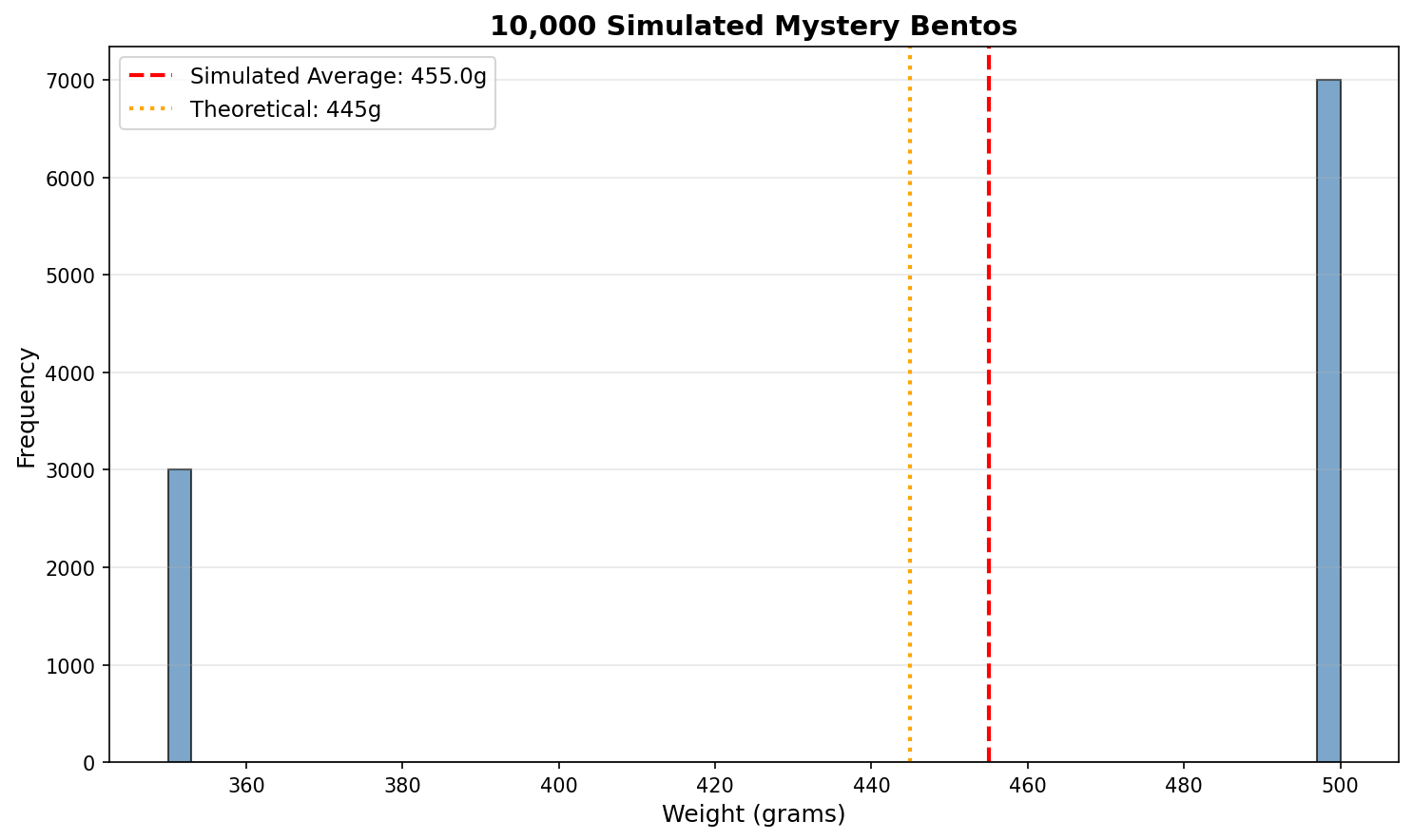
Output:

Observed average: 455.5g
Theoretical E[X]: 455.0g
Difference: 0.5g

Actual counts:
  Tonkatsu: 701 (70.1%)
  Hamburger: 299 (29.9%)

The long-run average converges to the expected value! This is the Law of Large Numbers in action.

Properties of Expected Value

Expected value has some useful mathematical properties that will be crucial for mixture models:

Linearity

Property 1: $E[aX + b] = aE[X] + b$

If you scale and shift a random variable, its expected value scales and shifts the same way.

Example: Chibany switches to measuring in ounces instead of grams. 1 gram ≈ 0.035 ounces, so weight in oz = weight in g × 0.035

$$E[\text{weight in oz}] = 0.035 \times E[\text{weight in g}] = 0.035 \times 455 \approx 15.9\text{ oz}$$

Property 2: $E[X + Y] = E[X] + E[Y]$

The expected value of a sum is the sum of expected values. This holds even if X and Y are dependent!

Example: If Chibany receives 5 bentos in one day, the expected total weight is: $$E[\text{total}] = E[X_1] + E[X_2] + E[X_3] + E[X_4] + E[X_5]$$ $$= 5 \times E[\text{single bento}] = 5 \times 455 = 2275\text{g}$$

Modeling the Mixture with GenJAX

Now let’s see how to express Chibany’s bento mixture as a generative model using GenJAX! This builds directly on what you learned in Tutorial 2.

The Generative Process

Recall from Tutorial 2 that we express random processes using generative functions. Here’s Chibany’s bento selection process:

 1
 2
 3
 4
 5
 6
 7
 8
 9
10
11
12
13
14
15
16

import jax
import jax.numpy as jnp
from genjax import gen, choice_map, simulate, Plot

@gen
def bento_mixture():
    """Generate a single bento weight from the mixture"""
    # Step 1: Choose the bento type
    # 70% chance of tonkatsu, 30% chance of hamburger
    is_tonkatsu = jnp.bernoulli(0.7) @ "type"

    # Step 2: Assign the weight based on type
    # (For now, we use exact weights - we'll add variation in Chapter 3!)
    weight = jnp.where(is_tonkatsu, 500.0, 350.0)

    return weight @ "weight"

What’s happening here?

1. jnp.bernoulli(0.7) flips a weighted coin: 70% True (tonkatsu), 30% False (hamburger)
2. @ "type" gives this random choice an address (like you learned in Tutorial 2, Chapter 3)
3. jnp.where(is_tonkatsu, 500.0, 350.0) returns 500g if tonkatsu, 350g if hamburger
4. @ "weight" addresses the final output

This is the generative model for Chibany’s bentos!

Simulating from the Model

Let’s simulate 1000 bentos and calculate the average weight, just like Chibany’s experiment:

 1
 2
 3
 4
 5
 6
 7
 8
 9
10
11
12
13
14
15
16
17
18
19
20
21
22
23
24
25
26
27
28

import jax.random as random

# Create a random key (GenJAX requires explicit randomness)
import jax.numpy as jnp

key = random.PRNGKey(42)

# Simulate 1000 bentos
n_bentos = 1000
weights = []

for i in range(n_bentos):
    key, subkey = random.split(key)
    trace = simulate(bento_mixture)(subkey)
    weights.append(trace.get_retval())

weights = jnp.array(weights)

# Calculate statistics
mean_weight = jnp.mean(weights)
n_tonkatsu = jnp.sum(weights == 500.0)
n_hamburger = jnp.sum(weights == 350.0)

print(f"Simulated average weight: {mean_weight:.1f}g")
print(f"Theoretical E[X]: {0.7 * 500 + 0.3 * 350:.1f}g")
print(f"\nCounts:")
print(f"  Tonkatsu (500g): {n_tonkatsu} ({n_tonkatsu/n_bentos*100:.1f}%)")
print(f"  Hamburger (350g): {n_hamburger} ({n_hamburger/n_bentos*100:.1f}%)")

Output:

Simulated average weight: 454.5g
Theoretical E[X]: 455.0g

Counts:
  Tonkatsu (500g): 691 (69.1%)
  Hamburger (350g): 309 (30.9%)

The simulated average is very close to the theoretical expected value!

Connecting to Expected Value

Remember the expected value formula: $$E[X] = 0.7 \times 500 + 0.3 \times 350 = 455\text{g}$$

GenJAX simulates this process:

1. Each simulation samples from the generative process
2. The average of many samples approximates the expected value
3. This is Monte Carlo estimation: using simulation to approximate mathematical expectations

Examining Individual Traces

One power of GenJAX is that we can inspect what the model generates. Let’s look at a few traces:

 1
 2
 3
 4
 5
 6
 7
 8
 9
10
11

# Generate and examine 5 bentos
key = random.PRNGKey(123)

for i in range(5):
    key, subkey = random.split(key)
    trace = simulate(bento_mixture)(subkey)

    bento_type = "Tonkatsu" if trace["type"] else "Hamburger"
    weight = trace.get_retval()

    print(f"Bento {i+1}: {bento_type:10s} → {weight:.0f}g")

Output:

Bento 1: Tonkatsu   → 500g
Bento 2: Hamburger  → 350g
Bento 3: Tonkatsu   → 500g
Bento 4: Tonkatsu   → 500g
Bento 5: Hamburger  → 350g

Each trace records both the type (the random choice) and the weight (the return value). This is the trace structure you learned about in Tutorial 2, Chapter 3!

Preview: What’s Missing?

This model captures the discrete mixture (tonkatsu vs. hamburger) but notice what it doesn’t capture:

• Real tonkatsu bentos don’t weigh exactly 500g - they vary (488g, 505g, 515g, etc.)
• Real hamburger bentos don’t weigh exactly 350g - they vary too (348g, 358g, 362g, etc.)

To model this within-category variation, we need:

1. Continuous distributions (Chapter 2)
2. Gaussian distributions (Chapter 3)
3. Gaussian mixtures (Chapter 5)

That’s where we’re headed!

But We’re Not Done Yet…

Chibany stares at their histogram. They understand the average now. 455g makes sense as a mixture. But something still bothers them.

Look at these two measurements:

• 488g (probably tonkatsu)
• 362g (probably hamburger)

But what about 425g? It’s right in the middle. Is it a heavy hamburger or a light tonkatsu?

And another thing: the weights aren’t exactly 500g and 350g. They vary! Some tonkatsu bentos weigh 520g, others 485g. Why?

Chibany realizes:

Discrete categories aren’t enough. Weight is CONTINUOUS.

There aren’t just two possible values (350g and 500g). There are infinitely many possible weights between 340g and 520g.

The histogram shows this: the data has spread within each category.

To handle this, Chibany needs a new kind of probability: continuous probability distributions.

And the most important continuous distribution? The Gaussian (also called the Normal distribution). That’s what creates the bell-curve shapes within each category.

But first, we need to understand the fundamental framework for handling continuous probability…

Summary

Practice Problems

Problem 1: Menu Expansion

Chibany’s students start bringing a third type of bento: sushi (600g). Now the proportions are:

• 50% tonkatsu (500g)
• 30% hamburger (350g)
• 20% sushi (600g)

What is the expected bento weight?

Problem 2: Multiple Bentos

If the proportions are 70% tonkatsu (500g) and 30% hamburger (350g), what is the expected total weight of 10 bentos?

Problem 3: Conceptual Challenge

Chibany observes that their bentos have E[X] = 455g. Their colleague receives bentos from a different cafeteria and also observes E[X] = 455g.

Does this mean they’re receiving the same distribution of bentos? Why or why not?