The Continuum: Continuous Probability

From Counting to Measuring

Chibany stares at their histogram. They understand expected value now. The 455g average makes sense as a mixture of 500g tonkatsu and 350g hamburger bentos.

But something still bothers them.

Look at these actual measurements from their first week:

Monday:    520g  (tonkatsu)
Tuesday:   348g  (hamburger)
Wednesday: 505g  (tonkatsu)
Thursday:   362g  (hamburger)
Friday:    488g  (tonkatsu)

The weights aren’t exactly 500g and 350g! They vary.

And here’s the deeper question: What’s the probability that a bento weighs exactly 505.000000… grams?

Chibany realizes: in Tutorial 1, they learned probability by counting discrete outcomes. But weight isn’t discrete. It’s continuous. There are infinitely many possible values between 340g and 520g.

How do you assign probabilities when there are infinitely many possibilities?

The Problem with Discrete Probability

Let’s see why the discrete approach breaks down.

In Tutorial 1, Chibany used this formula: $$P(\text{event}) = \frac{\text{# of outcomes in event}}{\text{# of total outcomes}}$$

This worked because there were finitely many outcomes:

• Outcome space: {tonkatsu, hamburger}
• $P(\text{tonkatsu}) = \frac{1}{2}$ if choosing randomly

But with continuous weight, this breaks:

• Outcome space: all real numbers between (say) 340g and 520g
• $P(\text{weight} = 505g \text{ exactly}) = \frac{1}{\infty} = 0$

Every specific weight has probability ZERO!

This seems wrong. Chibany definitely observed 505g. How can something that happened have zero probability?

The Resolution: Probability Density

The solution is to stop asking about exact values and start asking about ranges.

Instead of:

• ❌ “What’s P(weight = 505g)?” (answer: 0)

Ask:

• ✅ “What’s P(500g ≤ weight ≤ 510g)?” (answer: some positive number)

Key insight: In continuous probability, we measure area not count.

Probability Density Functions (PDFs)

A probability density function (PDF) is a function $p(x)$ that tells you the relative likelihood of different values.

Important properties:

1. $p(x) \geq 0$ for all $x$ (density is never negative)
2. $\int_{-\infty}^{\infty} p(x) , dx = 1$ (total probability is 1)
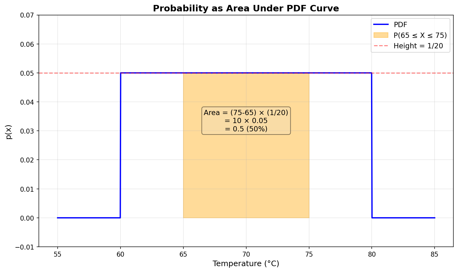
3. $P(a \leq X \leq b) = \int_a^b p(x) , dx$ (probability is area under curve)

Crucially: $p(x)$ itself is not a probability! It’s a density.

• $p(x)$ can be greater than 1
• Only the area under $p(x)$ is a probability

Visualizing PDF vs Probability

Let’s see this with a simple example: a uniform distribution from 0 to 1.

1
2
3
4
5
6
7

import jax.numpy as jnp
import matplotlib.pyplot as plt

# PDF: uniform from 0 to 1
# p(x) = 1 for 0 ≤ x ≤ 1, and 0 otherwise
x = jnp.linspace(-0.5, 1.5, 1000)
pdf = jnp.where((x >= 0) & (x <= 1), 1.0, 0.0)

 1
 2
 3
 4
 5
 6
 7
 8
 9
10
11
12
13
14
15
16
17
18
19
20
21
22
23
24
25
26
27
28
29
30
31
32

plt.figure(figsize=(12, 5))

# Plot 1: The PDF itself
plt.subplot(1, 2, 1)
plt.plot(x, pdf, 'b-', linewidth=2)
plt.fill_between(x, 0, pdf, alpha=0.3)
plt.xlabel('x', fontsize=12)
plt.ylabel('p(x)', fontsize=12)
plt.title('Probability Density Function', fontsize=14, fontweight='bold')
plt.ylim(-0.1, 1.3)
plt.grid(alpha=0.3)

# Plot 2: Probability of a range
plt.subplot(1, 2, 2)
plt.plot(x, pdf, 'b-', linewidth=2, alpha=0.3)

# Highlight the region 0.3 ≤ x ≤ 0.7
region_x = x[(x >= 0.3) & (x <= 0.7)]
region_pdf = pdf[(x >= 0.3) & (x <= 0.7)]
plt.fill_between(region_x, 0, region_pdf, color='orange', alpha=0.7,
                 label=f'P(0.3 ≤ X ≤ 0.7) = {0.7-0.3:.1f}')

plt.xlabel('x', fontsize=12)
plt.ylabel('p(x)', fontsize=12)
plt.title('Probability = Area Under Curve', fontsize=14, fontweight='bold')
plt.ylim(-0.1, 1.3)
plt.legend(fontsize=11)
plt.grid(alpha=0.3)

plt.tight_layout()
plt.savefig('visualization_1.png', dpi=150, bbox_inches='tight')
plt.show()

Key observations:

• The PDF is flat at height 1.0 (uniform density)
• $P(0.3 \leq X \leq 0.7) = \text{area} = \text{width} \times \text{height} = 0.4 \times 1.0 = 0.4$
• $P(X = 0.5 \text{ exactly}) = \text{area of vertical line} = 0$

The Uniform Distribution

The simplest continuous distribution is the uniform distribution.

Definition: A random variable $X$ is uniformly distributed on $[a, b]$ if all values in that range are equally likely.

PDF: $$p(x) = \begin{cases} \frac{1}{b-a} & \text{if } a \leq x \leq b \ 0 & \text{otherwise} \end{cases}$$

Intuition: The PDF is flat (constant) across the allowed range. The height is $\frac{1}{b-a}$ so that the total area equals 1.

In notation: $X \sim \text{Uniform}(a, b)$

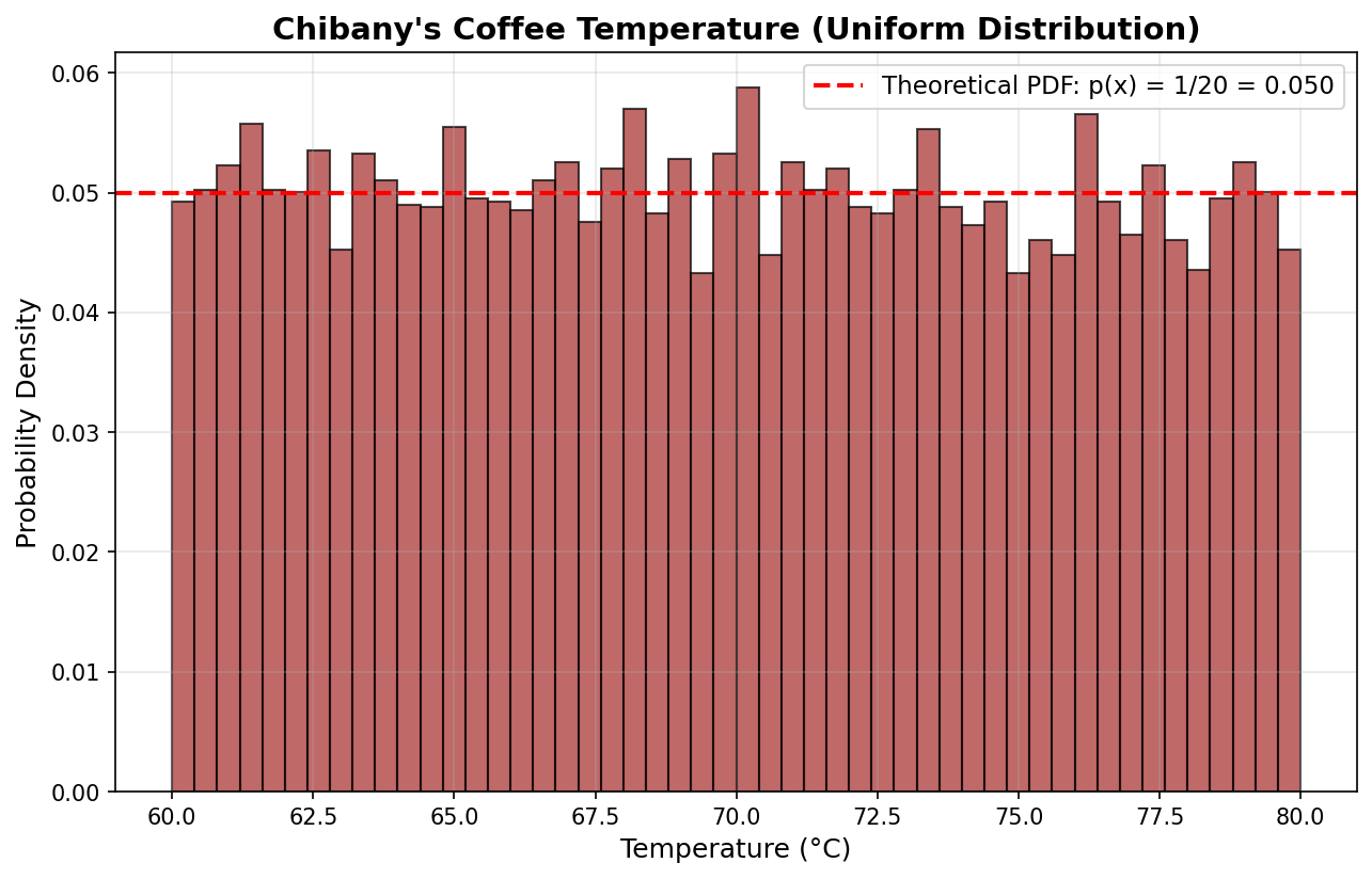
Example: Uniform Coffee Temperature

Chibany’s office coffee machine is unreliable. The temperature of their morning coffee is uniformly distributed between 60°C and 80°C.

 1
 2
 3
 4
 5
 6
 7
 8
 9
10
11
12
13
14
15
16
17
18
19
20

from genjax import gen, uniform
import jax.numpy as jnp
import jax.random as random

@gen
def coffee_temperature():
    """Model: coffee temperature uniformly between 60 and 80 degrees C"""
    temp = uniform(60.0, 80.0) @ "temp"
    return temp

# Simulate 10,000 cups
key = random.PRNGKey(42)
temps = []

for _ in range(10000):
    key, subkey = random.split(key)
    trace = coffee_temperature.simulate(subkey)
    temps.append(trace.get_retval())

temps = jnp.array(temps)

 1
 2
 3
 4
 5
 6
 7
 8
 9
10
11
12

# Plot histogram
plt.figure(figsize=(10, 6))
plt.hist(temps, bins=50, density=True, alpha=0.7, color='brown', edgecolor='black')
plt.axhline(1/(80-60), color='red', linestyle='--', linewidth=2,
            label=f'Theoretical PDF: p(x) = 1/20 = {1/20:.3f}')
plt.xlabel('Temperature (°C)', fontsize=12)
plt.ylabel('Probability Density', fontsize=12)
plt.title("Chibany's Coffee Temperature (Uniform Distribution)", fontsize=14, fontweight='bold')
plt.legend(fontsize=11)
plt.grid(alpha=0.3)
plt.savefig('coffee_temperature_histogram.png', dpi=150, bbox_inches='tight')
plt.show()

 1
 2
 3
 4
 5
 6
 7
 8
 9
10
11

# Continued from previous code block (requires temps array from above)
# Calculate probabilities for ranges
import jax.numpy as jnp

prob_too_cold = jnp.mean(temps < 65)  # Below 65°C
prob_just_right = jnp.mean((temps >= 70) & (temps <= 75))  # 70-75°C
prob_too_hot = jnp.mean(temps > 75)  # Above 75°C

print(f"P(temp < 65°C) = {prob_too_cold:.3f}")
print(f"P(70°C ≤ temp ≤ 75°C) = {prob_just_right:.3f}")
print(f"P(temp > 75°C) = {prob_too_hot:.3f}")

Output:

P(temp < 65°C) = 0.250
P(70°C ≤ temp ≤ 75°C) = 0.250
P(temp > 75°C) = 0.250

Theoretical calculation:

• $P(\text{temp} < 65) = \frac{65-60}{80-60} = \frac{5}{20} = 0.25$ ✓
• $P(70 \leq \text{temp} \leq 75) = \frac{75-70}{80-60} = \frac{5}{20} = 0.25$ ✓
• $P(\text{temp} > 75) = \frac{80-75}{80-60} = \frac{5}{20} = 0.25$ ✓

Perfect match! GenJAX simulations approximate the theoretical probabilities.

Cumulative Distribution Functions (CDFs)

Another way to work with continuous distributions is through the cumulative distribution function (CDF).

Definition: The CDF of a random variable $X$ is: $$F_X(x) = P(X \leq x) = \int_{-\infty}^x p(t) , dt$$

It tells you: “What’s the probability that X is at most x?”

Properties:

1. $F_X(-\infty) = 0$ (probability of being ≤ negative infinity is 0)
2. $F_X(\infty) = 1$ (probability of being ≤ infinity is 1)
3. $F_X$ is non-decreasing (never goes down)
4. $P(a \leq X \leq b) = F_X(b) - F_X(a)$ (subtract CDFs to get probabilities)

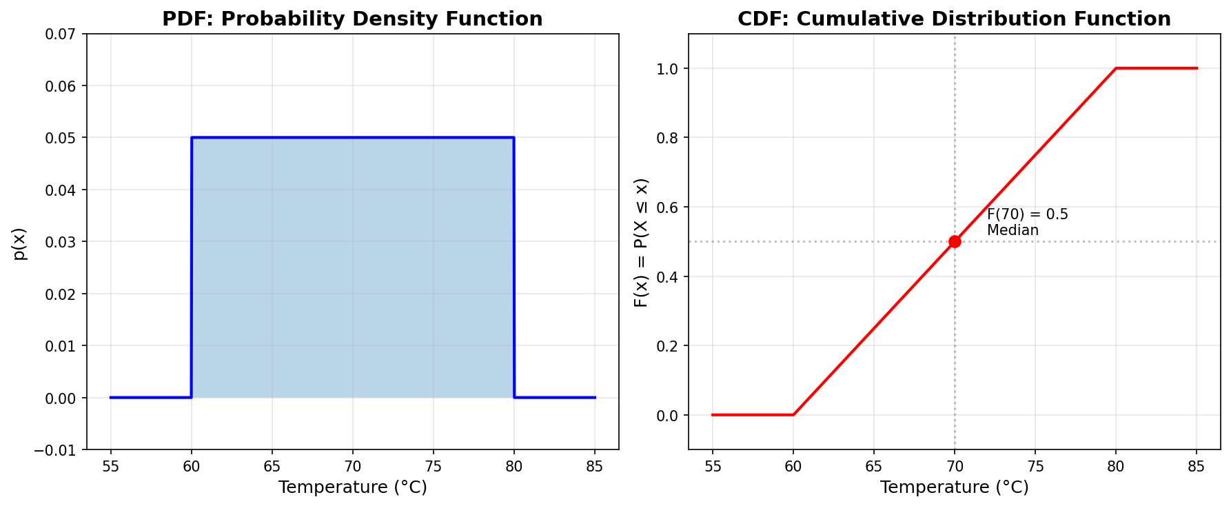
CDF for Uniform Distribution

For $X \sim \text{Uniform}(a, b)$:

$$F_X(x) = \begin{cases} 0 & \text{if } x < a \ \frac{x-a}{b-a} & \text{if } a \leq x \leq b \ 1 & \text{if } x > b \end{cases}$$

Let’s visualize this for Chibany’s coffee:

 1
 2
 3
 4
 5
 6
 7
 8
 9
10
11
12
13

import jax.numpy as jnp
import matplotlib.pyplot as plt

# Coffee temperature: Uniform(60, 80)
x = jnp.linspace(55, 85, 1000)

# PDF
pdf = jnp.where((x >= 60) & (x <= 80), 1/20, 0.0)

# CDF
cdf = jnp.where(x < 60, 0.0,
        jnp.where(x > 80, 1.0,
                  (x - 60) / 20))

 1
 2
 3
 4
 5
 6
 7
 8
 9
10
11
12
13
14
15
16
17
18
19
20
21
22
23
24
25
26
27
28
29
30

plt.figure(figsize=(12, 5))

# Plot 1: PDF
plt.subplot(1, 2, 1)
plt.plot(x, pdf, 'b-', linewidth=2)
plt.fill_between(x, 0, pdf, alpha=0.3)
plt.xlabel('Temperature (°C)', fontsize=12)
plt.ylabel('p(x)', fontsize=12)
plt.title('PDF: Probability Density Function', fontsize=14, fontweight='bold')
plt.ylim(-0.01, 0.07)
plt.grid(alpha=0.3)

# Plot 2: CDF
plt.subplot(1, 2, 2)
plt.plot(x, cdf, 'r-', linewidth=2)
plt.xlabel('Temperature (°C)', fontsize=12)
plt.ylabel('F(x) = P(X ≤ x)', fontsize=12)
plt.title('CDF: Cumulative Distribution Function', fontsize=14, fontweight='bold')
plt.ylim(-0.1, 1.1)
plt.grid(alpha=0.3)

# Mark special points
plt.axhline(0.5, color='gray', linestyle=':', alpha=0.5)
plt.axvline(70, color='gray', linestyle=':', alpha=0.5)
plt.plot(70, 0.5, 'ro', markersize=8)
plt.text(72, 0.52, 'F(70) = 0.5\nMedian', fontsize=10)

plt.tight_layout()
plt.savefig('pdf_vs_cdf.png', dpi=150, bbox_inches='tight')
plt.show()

Reading the CDF:

• At x = 70°C, F(70) = 0.5: “50% of coffees are ≤ 70°C”
• At x = 65°C, F(65) = 0.25: “25% of coffees are ≤ 65°C”
• At x = 75°C, F(75) = 0.75: “75% of coffees are ≤ 75°C”

Connecting Back to Chibany’s Bentos

Remember Chibany’s observation: bento weights aren’t exactly 500g and 350g - they vary!

Now we have the tools to model this variation:

1. Tonkatsu bentos: Weight is continuous around 500g
2. Hamburger bentos: Weight is continuous around 350g

But a uniform distribution doesn’t fit. Why?

• Uniform says all values equally likely in a range
• But we see weights cluster near 500g and 350g
• Values far from the center are less likely

We need a distribution that:

• Has a peak (mode) at the center
• Gets less likely as you move away
• Has controlled spread (some bentos vary more than others)

That distribution is the Gaussian (Normal) distribution - the famous bell curve!

That’s what we’ll study in the next chapter.

Summary

Practice Problems

Problem 1: Waiting Time

Chibany’s bus arrives uniformly between 8:00 AM and 8:20 AM. What’s the probability it arrives:

• a) Before 8:05 AM?
• b) Between 8:10 AM and 8:15 AM?
• c) After 8:18 AM?

Problem 2: GenJAX Simulation

Write a GenJAX generative function for Problem 1 and simulate 10,000 bus arrivals. Verify that your empirical probabilities match the theoretical values.

 1
 2
 3
 4
 5
 6
 7
 8
 9
10
11
12
13
14
15
16
17
18
19
20
21
22
23
24
25
26
27
28
29

from genjax import gen, uniform
import jax.numpy as jnp
import jax.random as random

@gen
def bus_arrival():
    """Bus arrives uniformly between 0 and 20 minutes after 8:00 AM"""
    arrival_time = uniform(0.0, 20.0) @ "arrival"
    return arrival_time

# Simulate 10,000 arrivals
key = random.PRNGKey(123)
arrivals = []

for _ in range(10000):
    key, subkey = random.split(key)
    trace = bus_arrival.simulate(subkey)
    arrivals.append(trace.get_retval())

arrivals = jnp.array(arrivals)

# Calculate empirical probabilities
prob_before_5 = jnp.mean(arrivals < 5)
prob_10_to_15 = jnp.mean((arrivals >= 10) & (arrivals <= 15))
prob_after_18 = jnp.mean(arrivals > 18)

print(f"a) P(before 8:05): {prob_before_5:.3f} (theoretical: 0.250)")
print(f"b) P(8:10 to 8:15): {prob_10_to_15:.3f} (theoretical: 0.250)")
print(f"c) P(after 8:18): {prob_after_18:.3f} (theoretical: 0.100)")

a) P(before 8:05): 0.248 (theoretical: 0.250)
b) P(8:10 to 8:15): 0.252 (theoretical: 0.250)
c) P(after 8:18): 0.099 (theoretical: 0.100)

Problem 3: Why Zero Probability Doesn’t Mean Impossible

If $P(X = 505.0 \text{ exactly}) = 0$, how is it possible that Chibany observed a bento weighing exactly 505.0g?

Next: Chapter 3 - The Gaussian Distribution →

Where we finally meet the bell curve and understand why it’s everywhere in nature!