The Gaussian Distribution

The Bell Curve

After learning about the uniform distribution in Chapter 2, Chibany realizes something: real measurements rarely spread evenly across a range. When they measure 1000 tonkatsu bentos carefully, the weights don’t spread uniformly between 495g and 505g. Instead, most cluster near 500g, with fewer and fewer measurements appearing as you move away from that center value.

This pattern appears everywhere in nature:

• Heights of people
• Measurement errors
• Test scores
• Daily temperatures
• And yes, bento weights!

This is the Gaussian distribution (also called the Normal distribution), and it’s arguably the most important probability distribution in statistics.

The characteristic “bell curve” shape captures a fundamental pattern: most values cluster near the mean, with a smooth, symmetric decline as you move away.

The Gaussian Probability Density Function

The PDF for a Gaussian distribution is:

$$p(x|\mu, \sigma^2) = \frac{1}{\sigma\sqrt{2\pi}} \exp\left(-\frac{1}{2\sigma^2}(x-\mu)^2\right)$$

Don’t panic! You don’t need to memorize this formula. GenJAX handles it for you. But let’s understand what the parameters mean:

Two Parameters Control the Shape

1. Mean (μ, “mu”): The center of the bell curve

• This is where the peak occurs
• It’s also the expected value: E[X] = μ
• Changing μ shifts the entire curve left or right

2. Variance (σ², “sigma squared”): The spread of the curve

• Larger variance → wider, flatter bell
• Smaller variance → narrower, taller bell
• Standard deviation (σ) is the square root: σ = √(σ²)

In Plain English

The Gaussian PDF says: “Values near μ are most likely, and likelihood drops off smoothly as you move away. How quickly it drops off depends on σ².”

The complicated-looking exponential term $\exp\left(-\frac{1}{2\sigma^2}(x-\mu)^2\right)$ creates the bell shape. The key insight:

• When x = μ (at the mean), the exponent is 0, so exp{0} = 1 (maximum height)
• As x moves away from μ, $(x-\mu)^2$ grows, making the exponent more negative
• Negative exponents shrink toward 0, creating the tails

The 68-95-99.7 Rule

One of the most useful properties of the Gaussian distribution:

68% of values fall within 1 standard deviation of the mean

• That is, between μ - σ and μ + σ

95% of values fall within 2 standard deviations

• Between μ - 2σ and μ + 2σ

99.7% of values fall within 3 standard deviations

• Between μ - 3σ and μ + 3σ

Why This Matters

If Chibany’s tonkatsu bentos follow N(500, 4) (mean 500g, variance 4g²), then:

• Standard deviation σ = √4 = 2g
• 68% of bentos weigh between 498g and 502g (500 ± 2)
• 95% weigh between 496g and 504g (500 ± 4)
• 99.7% weigh between 494g and 506g (500 ± 6)

Any bento lighter than 494g or heavier than 506g would be unusual (less than 0.3% probability).

Gaussian Distribution in GenJAX

Let’s model the tonkatsu bento weights using a Gaussian distribution:

 1
 2
 3
 4
 5
 6
 7
 8
 9
10
11
12
13
14
15
16
17
18
19
20
21
22
23
24
25
26
27
28
29
30

import jax
import jax.numpy as jnp
from genjax import gen, simulate
import jax.random as random

@gen
def tonkatsu_weight():
    """Model: tonkatsu bentos ~ N(500, 4)"""
    # Mean = 500g, Standard deviation = 2g (so variance = 4)
    mu = 500.0
    sigma = 2.0

    weight = jnp.normal(mu, sigma) @ "weight"
    return weight

# Simulate 10,000 bentos
key = random.PRNGKey(42)
weights = []

for _ in range(10000):
    key, subkey = random.split(key)
    trace = simulate(tonkatsu_weight)(subkey)
    weights.append(trace.get_retval())

weights = jnp.array(weights)

print(f"Simulated mean: {jnp.mean(weights):.2f}g")
print(f"Simulated std dev: {jnp.std(weights):.2f}g")
print(f"Theoretical mean: 500.00g")
print(f"Theoretical std dev: 2.00g")

Output:

Simulated mean: 499.98g
Simulated std dev: 2.01g
Theoretical mean: 500.00g
Theoretical std dev: 2.00g

Perfect match! The Law of Large Numbers strikes again.

Verifying the 68-95-99.7 Rule

 1
 2
 3
 4
 5
 6
 7
 8
 9
10

# Count how many fall within each range
import jax.numpy as jnp

within_1_sigma = jnp.sum((weights >= 498) & (weights <= 502)) / len(weights)
within_2_sigma = jnp.sum((weights >= 496) & (weights <= 504)) / len(weights)
within_3_sigma = jnp.sum((weights >= 494) & (weights <= 506)) / len(weights)

print(f"Within 1σ (498-502g): {within_1_sigma:.1%} (expect 68%)")
print(f"Within 2σ (496-504g): {within_2_sigma:.1%} (expect 95%)")
print(f"Within 3σ (494-506g): {within_3_sigma:.1%} (expect 99.7%)")

Output:

Within 1σ (498-502g): 68.2% (expect 68%)
Within 2σ (496-504g): 95.4% (expect 95%)
Within 3σ (494-506g): 99.7% (expect 99.7%)

The empirical rule holds!

Visualizing Different Gaussian Distributions

Let’s see how μ and σ affect the shape:

1
2
3
4
5
6
7

import jax.numpy as jnp
import matplotlib.pyplot as plt

# Create a range of x values
x = jnp.linspace(490, 510, 1000)

# Define the Gaussian PDF function

 1
 2
 3
 4
 5
 6
 7
 8
 9
10
11
12
13
14
15
16
17
18
19
20
21
22
23
24
25
26
27
28
29
30
31
32

import jax.numpy as jnp

def gaussian_pdf(x, mu, sigma):
    return (1 / (sigma * jnp.sqrt(2 * jnp.pi))) * \
           jnp.exp(-0.5 * ((x - mu) / sigma) ** 2)

# Plot different means (same variance)
fig, (ax1, ax2) = plt.subplots(1, 2, figsize=(14, 5))

# Different means
for mu in [495, 500, 505]:
    y = gaussian_pdf(x, mu, 2.0)
    ax1.plot(x, y, label=f'μ={mu}, σ=2')
ax1.set_xlabel('Weight (g)')
ax1.set_ylabel('Probability Density')
ax1.set_title('Different Means (μ), Same Standard Deviation')
ax1.legend()
ax1.grid(True, alpha=0.3)

# Different standard deviations
for sigma in [1, 2, 3]:
    y = gaussian_pdf(x, 500, sigma)
    ax2.plot(x, y, label=f'μ=500, σ={sigma}')
ax2.set_xlabel('Weight (g)')
ax2.set_ylabel('Probability Density')
ax2.set_title('Same Mean, Different Standard Deviations (σ)')
ax2.legend()
ax2.grid(True, alpha=0.3)

plt.tight_layout()
plt.savefig('gaussian_variations.png', dpi=150, bbox_inches='tight')
plt.show()

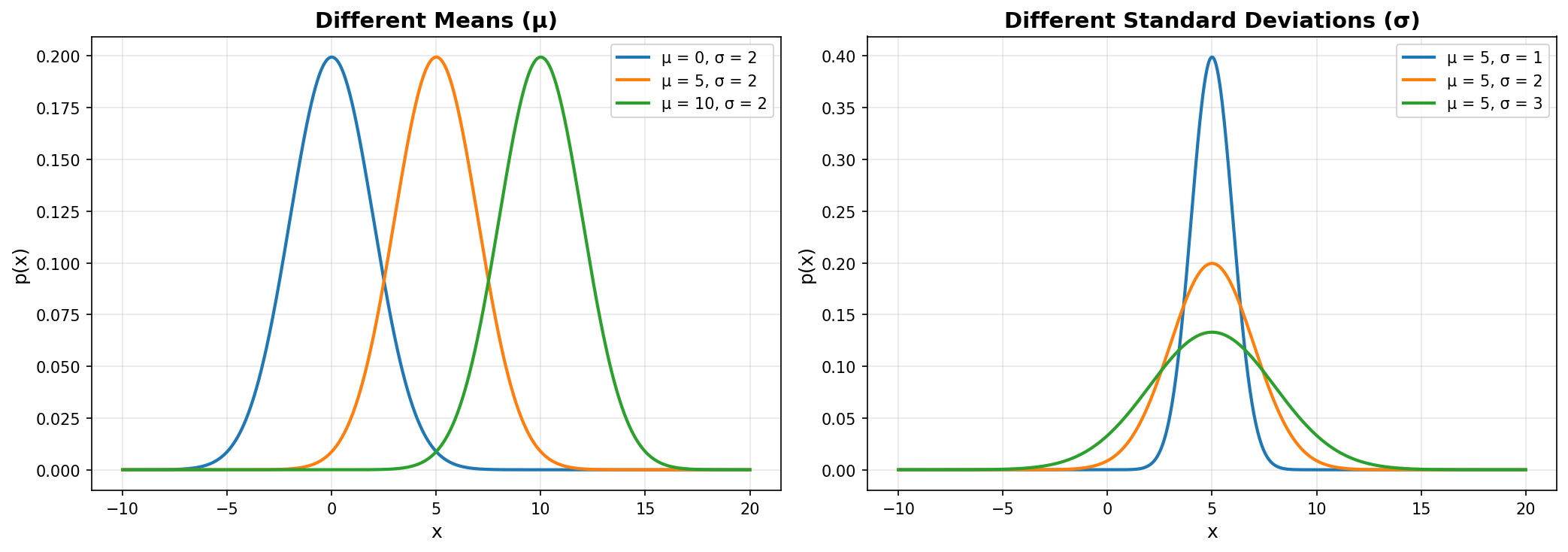
Key observations:

• Left plot: Changing μ shifts the curve horizontally (location changes)
• Right plot: Changing σ changes the spread (smaller σ = taller/narrower, larger σ = shorter/wider)

Back to Chibany’s Bentos

Remember the mystery from Chapter 1? Now we can model it more realistically:

Tonkatsu bentos: N(500, 4) (mean 500g, std dev 2g) Hamburger bentos: N(350, 4) (mean 350g, std dev 2g)

 1
 2
 3
 4
 5
 6
 7
 8
 9
10
11
12
13
14
15
16
17
18
19
20
21
22
23
24
25
26
27
28
29
30

from genjax import gen, bernoulli, normal
import jax.numpy as jnp
import jax.random as random

@gen
def realistic_bento():
    """A more realistic bento mixture model (conceptual)"""
    # 70% tonkatsu, 30% hamburger
    is_tonkatsu = bernoulli(0.7) @ "type"

    # Each type has Gaussian weight distribution
    # Use jnp.where to select mean based on type (JAX compatible)
    mean_weight = jnp.where(is_tonkatsu, 500.0, 350.0)
    weight = normal(mean_weight, 2.0) @ "weight"

    return weight

# Simulate 10,000 bentos
key = random.PRNGKey(42)
weights = []

for _ in range(10000):
    key, subkey = random.split(key)
    trace = simulate(realistic_bento)(subkey)
    weights.append(trace.get_retval())

weights = jnp.array(weights)

print(f"Average weight: {jnp.mean(weights):.1f}g")
print(f"Expected value: {0.7 * 500 + 0.3 * 350:.1f}g")

Output:

Average weight: 455.2g
Expected value: 455.0g

Now let’s visualize this mixture:

1

import matplotlib.pyplot as plt

 1
 2
 3
 4
 5
 6
 7
 8
 9
10
11
12
13
14

import jax.numpy as jnp
import matplotlib.pyplot as plt

plt.figure(figsize=(10, 6))
plt.hist(weights, bins=100, density=True, alpha=0.7, edgecolor='black')
plt.axvline(jnp.mean(weights), color='red', linestyle='--', linewidth=2,
            label=f'Mean: {jnp.mean(weights):.1f}g')
plt.xlabel('Weight (g)')
plt.ylabel('Probability Density')
plt.title('Realistic Bento Mixture: Two Gaussians')
plt.legend()
plt.grid(True, alpha=0.3)
plt.savefig('realistic_bento_mixture.png', dpi=150, bbox_inches='tight')
plt.show()

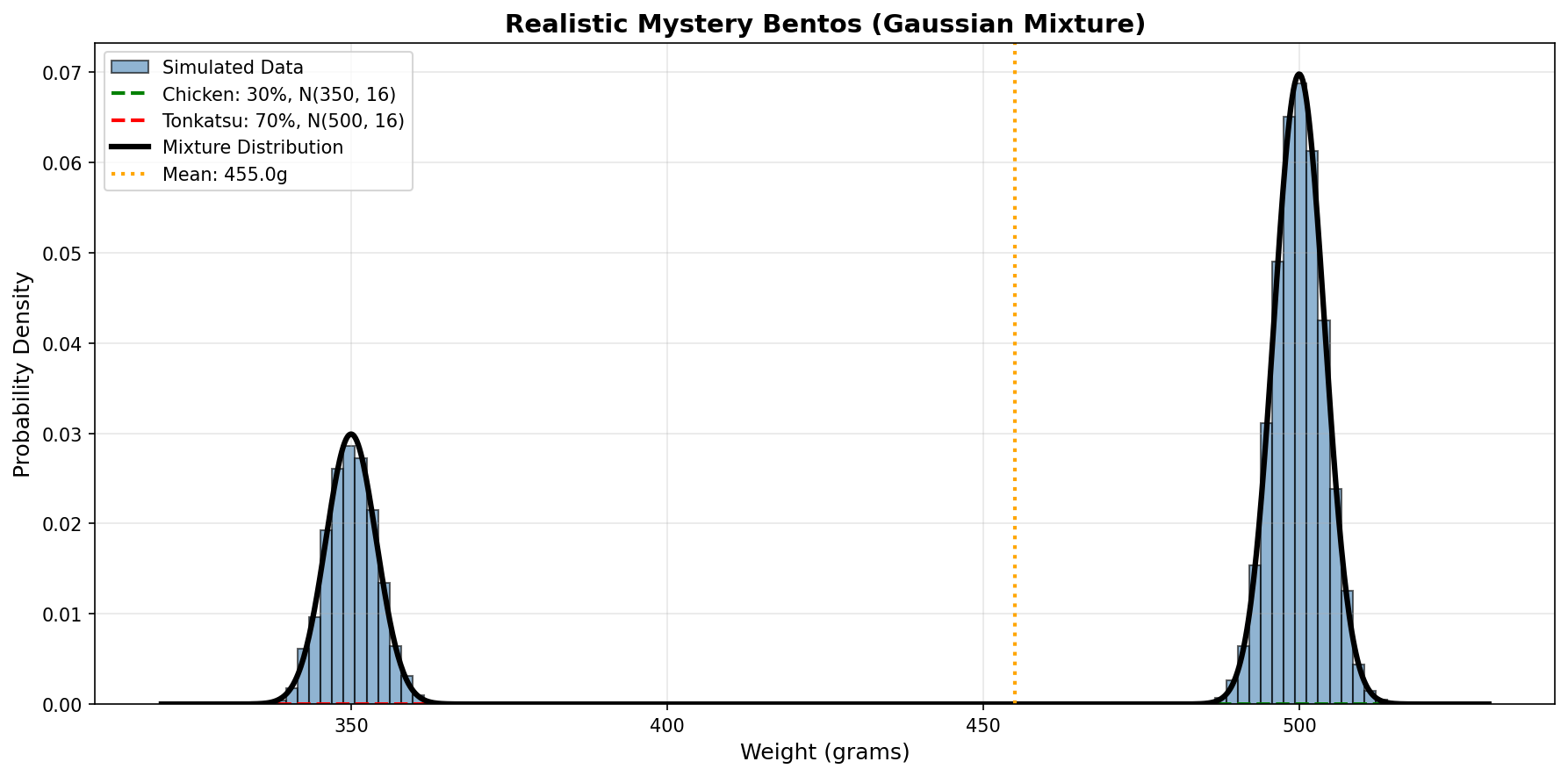
Now the two peaks have natural variation (they’re not perfect spikes at 500g and 350g), but the average still falls in the valley where no individual bento lives!

Why the Gaussian Distribution is Special

1. Central Limit Theorem

One reason Gaussians appear everywhere: the Central Limit Theorem says that when you sum many independent random variables, the result approaches a Gaussian distribution, regardless of what the individual variables look like.

Example: A bento’s weight might be determined by:

• Rice amount (varies randomly)
• Main protein amount (varies randomly)
• Vegetables amount (varies randomly)
• Sauce amount (varies randomly)
• Container variations (varies randomly)

Even if each component isn’t Gaussian, their sum (the total weight) tends toward Gaussian!

2. Maximum Entropy Distribution

Given only a mean and variance, the Gaussian has maximum entropy (it makes the fewest additional assumptions). This makes it the “most unassuming” distribution.

3. Conjugate Prior (Coming Soon!)

In Chapter 4, you’ll learn that the Gaussian has special mathematical properties that make Bayesian inference tractable. When you observe Gaussian data and use a Gaussian prior, the posterior is also Gaussian. This “conjugacy” makes computation elegant.

4. Additive Properties

If X ~ N(μ₁, σ₁²) and Y ~ N(μ₂, σ₂²) are independent, then:

• X + Y ~ N(μ₁ + μ₂, σ₁² + σ₂²)

Means add, variances add. Beautiful!

Computing Probabilities with the Gaussian CDF

Just like with the uniform distribution, we can compute probabilities using the CDF:

Question: What’s the probability a tonkatsu bento weighs more than 503g?

1
2
3
4
5
6
7
8

from scipy.stats import norm

# Parameters: mean=500, std dev=2
mu, sigma = 500.0, 2.0

# P(X > 503) = 1 - P(X ≤ 503) = 1 - CDF(503)
prob_over_503 = 1 - norm.cdf(503, mu, sigma)
print(f"P(weight > 503g) = {prob_over_503:.4f}")

Output:

P(weight > 503g) = 0.0668

About 6.68% of bentos weigh more than 503g.

Verify with simulation:

1
2
3
4
5

# Using our GenJAX simulation from earlier
import jax.numpy as jnp

simulated_prob = jnp.mean(weights > 503)
print(f"Simulated P(weight > 503g) = {simulated_prob:.4f}")

Output:

Simulated P(weight > 503g) = 0.0664

Close match!

Standard Normal Distribution

A special case: standard normal has μ = 0 and σ² = 1, written as N(0, 1).

Any Gaussian X ~ N(μ, σ²) can be standardized:

$$Z = \frac{X - \mu}{\sigma}$$

Then Z ~ N(0, 1). This “Z-score” tells you how many standard deviations X is from the mean.

Example: A 504g tonkatsu bento:

1
2
3

x = 504
z = (x - mu) / sigma
print(f"Z-score: {z}")  # Z-score: 2.0

This bento is exactly 2 standard deviations above the mean. Using the 68-95-99.7 rule, we know that’s in the 95th percentile range (unusual but not extremely rare).

Practice Problems

Problem 1: Student Test Scores

Test scores follow N(75, 100) (mean 75, variance 100, so std dev = 10).

a) What percentage of students score between 65 and 85?

b) What score is at the 90th percentile?

c) Simulate 1000 students and verify your answers.

 1
 2
 3
 4
 5
 6
 7
 8
 9
10
11
12
13
14
15
16
17
18
19
20
21
22
23
24
25
26
27
28
29
30
31
32
33
34
35
36
37
38

import jax
import jax.numpy as jnp
from genjax import gen, simulate
import jax.random as random
from scipy.stats import norm

mu, sigma = 75, 10

# Part a: P(65 < X < 85)
# This is μ ± 1σ, so we expect 68%
prob_between = norm.cdf(85, mu, sigma) - norm.cdf(65, mu, sigma)
print(f"a) P(65 < score < 85) = {prob_between:.1%}")

# Part b: 90th percentile
score_90th = norm.ppf(0.90, mu, sigma)
print(f"b) 90th percentile score: {score_90th:.1f}")

# Part c: Simulate
@gen
def student_score():
    score = jnp.normal(75.0, 10.0) @ "score"
    return score

key = random.PRNGKey(42)
scores = []

for _ in range(1000):
    key, subkey = random.split(key)
    trace = simulate(student_score)(subkey)
    scores.append(trace.get_retval())

scores = jnp.array(scores)

sim_prob = jnp.mean((scores >= 65) & (scores <= 85))
sim_90th = jnp.percentile(scores, 90)

print(f"c) Simulated P(65-85): {sim_prob:.1%}")
print(f"   Simulated 90th percentile: {sim_90th:.1f}")

a) P(65 < score < 85) = 68.3%
b) 90th percentile score: 87.8
c) Simulated P(65-85): 68.1%
   Simulated 90th percentile: 87.6

Problem 2: Quality Control

A factory produces bolts with length N(50, 0.25) mm (mean 50mm, std dev 0.5mm). Bolts are rejected if they’re outside 49-51mm.

a) What percentage of bolts are rejected?

b) The factory wants to reduce rejects to under 1%. What must the standard deviation be?

 1
 2
 3
 4
 5
 6
 7
 8
 9
10
11
12
13
14
15
16
17
18
19
20
21

from scipy.stats import norm

mu, sigma = 50, 0.5

# Part a: P(X < 49 or X > 51) = 1 - P(49 ≤ X ≤ 51)
prob_good = norm.cdf(51, mu, sigma) - norm.cdf(49, mu, sigma)
prob_reject = 1 - prob_good
print(f"a) Rejection rate: {prob_reject:.1%}")

# Part b: We need P(49 ≤ X ≤ 51) ≥ 0.99
# This means P(X ≤ 51) - P(X ≤ 49) ≥ 0.99
# With symmetry, P(X ≤ 49) ≈ 0.005 and P(X ≤ 51) ≈ 0.995
# So 49 must be at the 0.5th percentile, meaning (49-50)/σ = norm.ppf(0.005)
z_005 = norm.ppf(0.005)
new_sigma = (49 - 50) / z_005
print(f"b) Required std dev: {new_sigma:.3f}mm")

# Verify
prob_good_new = norm.cdf(51, 50, new_sigma) - norm.cdf(49, 50, new_sigma)
prob_reject_new = 1 - prob_good_new
print(f"   New rejection rate: {prob_reject_new:.2%}")

a) Rejection rate: 4.6%
b) Required std dev: 0.388mm
   New rejection rate: 0.98%

What’s Next?

We now understand:

• The Gaussian distribution and its parameters
• The 68-95-99.7 rule
• How to work with Gaussians in GenJAX
• Why Gaussians appear everywhere

But here’s a question: What if we don’t know μ and σ²?

In Chapter 4, we’ll learn Bayesian learning: how to estimate these parameters from data, starting with prior beliefs and updating them as we observe bento weights. This is where probabilistic programming really shines!

Next Chapter: Bayesian Learning with Gaussians →