Dirichlet Process Mixture Models
The Problem with Fixed K
In Chapter 5, we solved Chibany’s bento mystery using a Gaussian Mixture Model (GMM) with K=2 components. But we had to specify K in advance and use BIC to validate our choice.
What if:
- We don’t know how many types exist?
- The number of types changes over time?
- We want the model to discover the number of clusters automatically?
Enter the Dirichlet Process Mixture Model (DPMM): A Bayesian nonparametric approach that learns the number of components from the data.
The Intuition: Infinite Clusters
Imagine Chibany’s supplier keeps adding new bento types over time. With a fixed-K GMM, they’d have to:
- Notice a new type appeared
- Re-run model selection (BIC) to choose new K
- Refit the entire model
With a DPMM, the model automatically discovers new clusters as data arrives, without needing to specify K upfront.
Key insight: The DPMM places a prior over an infinite number of potential clusters, but only a finite number will actually be “active” (have observations assigned to them).
The Chinese Restaurant Process Analogy
The most intuitive way to understand the DPMM is through the Chinese Restaurant Process (CRP).
The Setup
Imagine a restaurant with infinitely many tables (each table represents a cluster). Customers (observations) enter one by one and choose where to sit:
Rule: Customer n+1 sits:
- At an occupied table k with probability proportional to the number of customers already there: $\frac{n_k}{n + \alpha}$
- At a new table with probability: $\frac{\alpha}{n + \alpha}$
Where:
- nₖ = number of customers at table k
- α = “concentration parameter” (controls tendency to create new tables)
- n = total customers so far
The Rich Get Richer
This creates a rich-get-richer dynamic:
- Popular tables attract more customers (clustering)
- But there’s always a chance of starting a new table (flexibility)
- α controls the trade-off: larger α → more new tables
Connecting to Bentos
- Customer = bento observation
- Table = cluster (bento type)
- Seating choice = cluster assignment
- α = how likely new bento types appear
The Math: Stick-Breaking Construction
The DPMM uses a stick-breaking construction to define mixing proportions for infinitely many components.
The Process
Imagine a stick of length 1. We break it into pieces:
For k = 1, 2, 3, …, ∞:
- Sample βₖ ~ Beta(1, α)
- Set πₖ = βₖ × (1 - π₁ - π₂ - … - πₖ₋₁)
In plain English:
- β₁ = fraction of stick we take for component 1
- Remaining stick: 1 - β₁
- β₂ = fraction of remaining stick we take for component 2
- π₂ = β₂ × (1 - π₁)
- And so on…
Result: π₁, π₂, π₃, … sum to 1 (they’re valid mixing proportions), with later components getting exponentially smaller shares.
The Beta Distribution
βₖ ~ Beta(1, α) determines how much of the remaining stick we take:
- α large (e.g., α=10): Breaks are more even → many components with similar weights
- α small (e.g., α=0.5): First few breaks take most of the stick → few dominant components
DPMM for Gaussian Mixtures: The Full Model
Model Specification
Stick-breaking (infinite components):
- For k = 1, 2, …, K_max:
- βₖ ~ Beta(1, α)
- π₁ = β₁
- πₖ = βₖ × (1 - Σⱼ₌₁ᵏ⁻¹ πⱼ) for k > 1
Component parameters:
- μₖ ~ N(μ₀, σ₀²) [prior on means]
Observations (using stick-breaking weights directly):
- For i = 1, …, N:
- zᵢ ~ Categorical(π) [cluster assignment using stick-breaking weights]
- xᵢ ~ N(μ_zᵢ, σₓ²) [observation from assigned cluster]
Important: We use the stick-breaking weights π directly for cluster assignment. Adding an extra Dirichlet draw would create “double randomization” that makes inference much slower and less accurate!
Why K_max?
In practice, we truncate the infinite model at some large K_max (e.g., 10 or 20). As long as K_max > the true number of clusters, this approximation is accurate.
Implementing DPMM in GenJAX
Let’s implement the DPMM for Chibany’s bentos using the corrected approach:
| |
Output:
Generated data: [-10.4  -9.9 -10.1   0.1   9.9  10.2 ...]
Cluster assignments: [0, 0, 0, 5, 3, 3, 3, ...]
Notice: The model automatically discovered active clusters (0, 3, 5 in this run), ignoring the others!
Inference: A Slice Sampler for the DPMM
Now let’s condition on Chibany’s actual bento weights and infer the clusters. This is harder than the forward direction, and the choice of inference algorithm matters a lot.
Why not plain importance sampling?
The tempting first idea is to sample whole DPMMs from the prior and keep the ones that match the data (importance/rejection sampling). It fails badly here: a random 10-component stick-breaking draw almost never places its means near three tight clusters at $-10, 0, +10$, so essentially every sample gets a vanishingly small weight. We need an algorithm that moves toward the data instead of guessing blindly.
The slice-sampling idea
The classic solution is the slice sampler of Walker (2007). Its trick is to introduce one auxiliary “slice” variable per observation:
$$u_i \sim \text{Uniform}(0,\ \pi_{z_i})$$
where $\pi_{z_i}$ is the mixing weight of the cluster $i$ currently belongs to, and $\text{Uniform}(a,b)$ is the uniform distribution on the interval $[a,b]$.
Why is this useful? Given the slice values, a component $k$ is only a candidate for observation $i$ if its weight clears the slice, $\pi_k > u_i$. Because the stick-breaking weights shrink geometrically, only finitely many components ever clear the slice — so even though the model has infinitely many potential clusters, each sweep only has to consider a finite, adaptive set. The number of active clusters $K$ can grow or shrink from sweep to sweep as the data demand, which is exactly the behavior a nonparametric model should have. (We still allocate a generous truncation KMAX as a storage bound, but the slice — not the truncation — decides how many clusters are live.)
The Gibbs sweep
Each sweep cycles through four conditional updates, sampling each quantity given the current value of the others:
- Slice variables $u_i \sim \text{Uniform}(0, \pi_{z_i})$ — set the per-observation thresholds.
- Assignments $z_i$ — pick a cluster from those allowed by the slice, weighted by how well it explains $x_i$: $;P(z_i = k) \propto \mathbb{1}[\pi_k > u_i], \mathcal{N}(x_i \mid \mu_k, \sigma_x)$, where $\mathbb{1}[\cdot]$ is the indicator (1 if true, 0 if false).
- Stick weights $\beta_k \sim \text{Beta}(1 + n_k,\ \alpha + \sum_{j>k} n_j)$, where $n_k$ is the number of observations now in cluster $k$ — the standard stick-breaking posterior.
- Cluster means $\mu_k$ — a conjugate Normal–Normal update from the points assigned to cluster $k$ (empty clusters fall back to the prior).
We keep the explicit for-loops over sweeps so each step is readable; a later chapter shows how to vectorize with scan.
| |
Output:
=== DPMM slice sampler (300 sweeps, 100 burn-in, seed 0) ===
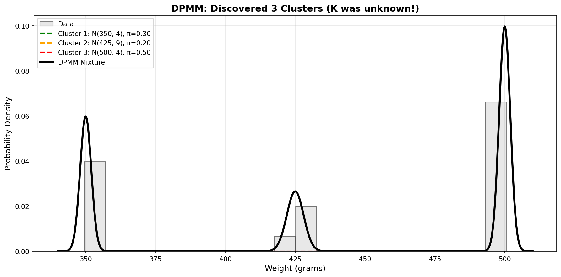
Discovered 3 active clusters
Cluster 0: mu = -10.03 (n = 5)
Cluster 1: mu = 0.29 (n = 1)
Cluster 2: mu = 10.25 (n = 5)
Posterior over number of clusters K:
P(K = 3) = 0.58
P(K = 4) = 0.35
P(K = 5) = 0.07The sampler recovers all three clusters — the five $\approx -10$ bentos, the lone $\approx 0$ bento, and the five $\approx +10$ bentos — and learns their means accurately. The posterior over $K$ also reflects genuine uncertainty in the number of clusters: $K=3$ is most probable, but the model gives real weight to a spurious fourth or fifth cluster — something a fixed-$K$ GMM cannot express at all.
A caveat: the posterior over $K$ is a treacherous object
It is tempting to read “$P(K = 3) = 0.58$” as the model’s calibrated belief about how many clusters really exist. Be careful — the marginal posterior over the number of clusters is a deep and nuanced object, and for the DPMM it does not behave the way you might hope.
Miller & Harrison (2014) proved that the DPMM’s posterior on the number of clusters is inconsistent: even when the data truly come from a finite mixture with a fixed number of components, as you collect more and more data the marginal posterior over $K$ keeps spawning extra clusters and never settles on the right number. Strikingly, this happens even while the model does density estimation perfectly well — the predictive distribution is fine, the joint is well-estimated; it is specifically the count $K$ that misbehaves. So a DPMM is an excellent density estimator and a treacherous cluster-counter.
The good news is that this is fixable, and the fix is one careful practitioners often reach for anyway. Ascolani, Lijoi, Rebaudo & Zanella (2022) showed that putting a prior on the concentration parameter $\alpha$ — rather than fixing it, as we did with ALPHA = 1.0 above — recovers consistency for the number of clusters when the data are generated from a finite mixture. Letting $\alpha$ itself be learned (the same “hyperprior on the prior” move you’ll see in Chapter 12) is exactly the elegant remedy. The practical upshot: trust the DPMM’s predictive fit and its clustering of the data, but treat any single number for “how many clusters” with suspicion unless you’ve put a prior on $\alpha$.
Slice values do the truncation
We allocated KMAX = 20 storage slots, but never assumed 20 clusters: in any sweep, only the components whose weight clears some observation’s slice ($\pi_k > u_i$) are live. The data, through the slice, decide how many clusters exist — which is the whole point of going nonparametric.
Analyzing the Posterior
The sampler gives us a collection of clusterings (one per post-burn-in sweep), not a single answer. Summarizing them takes a little care because of label switching: the cluster we call “0” in one sweep might be called “2” in the next, since the labels are arbitrary. So we cannot just average mu_0 across sweeps — that average mixes different physical clusters together and is meaningless.
Two summaries that are meaningful:
(1) A single representative clustering — take the final sweep and relabel its clusters left-to-right by their mean, so the numbering is interpretable:
| |
Output:
Cluster assignment per bento: [0, 0, 0, 0, 0, 1, 2, 2, 2, 2, 2]

Cluster means:
  Cluster 0: μ = -10.03   (n = 5)
  Cluster 1: μ =   0.29   (n = 1)
  Cluster 2: μ =  10.25   (n = 5)
(2) A label-invariant summary — the co-clustering probability that two bentos land in the same cluster, averaged over all samples. This sidesteps label switching entirely, because “same cluster?” doesn’t depend on what the cluster is named:
| |
Output:
Co-clustering probability matrix P(i ~ j):
  [1.00 0.92 0.90 0.88 0.90 0.00 0.00 0.00 0.00 0.00 0.00]
  [0.92 1.00 0.88 0.87 0.93 0.00 0.00 0.00 0.00 0.00 0.00]
  [0.90 0.88 1.00 0.88 0.88 0.00 0.00 0.00 0.00 0.00 0.00]
  [0.88 0.87 0.88 1.00 0.90 0.00 0.00 0.00 0.00 0.00 0.00]
  [0.90 0.93 0.88 0.90 1.00 0.00 0.00 0.00 0.00 0.00 0.00]
  [0.00 0.00 0.00 0.00 0.00 1.00 0.00 0.00 0.00 0.00 0.00]
  [0.00 0.00 0.00 0.00 0.00 0.00 1.00 0.90 0.93 0.90 0.86]
  [0.00 0.00 0.00 0.00 0.00 0.00 0.90 1.00 0.88 0.86 0.90]
  [0.00 0.00 0.00 0.00 0.00 0.00 0.93 0.88 1.00 0.88 0.90]
  [0.00 0.00 0.00 0.00 0.00 0.00 0.90 0.86 0.88 1.00 0.86]
  [0.00 0.00 0.00 0.00 0.00 0.00 0.86 0.90 0.90 0.86 1.00]
The block structure is unmistakable: the five $\approx -10$ bentos (rows 0–4) almost always share a cluster with each other and never with the rest; the lone $\approx 0$ bento (row 5) sits by itself; the five $\approx +10$ bentos (rows 6–10) form the third block. The model recovered the three groups without ever being told there were three — and the within-block probabilities sitting a little below 1.0 honestly reflect the small chance, seen in the posterior over $K$, that a group occasionally splits.
A Trap: Label Switching
We sidestepped a subtle but important problem above, and it’s worth making explicit because it bites every mixture model, not just the DPMM.
The cluster labels are arbitrary. Nothing in the model distinguishes “cluster 0” from “cluster 2” — the likelihood $$p(x \mid z, \mu) = \prod_i \mathcal{N}(x_i \mid \mu_{z_i}, \sigma_x)$$ is completely unchanged if we swap the names of two clusters and swap their means to match. The model has a built-in symmetry: with $K$ occupied clusters there are $K!$ equivalent labelings of the same clustering, all with identical posterior probability.
Why this breaks naive summaries. A good sampler will, over many sweeps, wander between these equivalent labelings — the group sitting at $-10$ might be called cluster 0 in one sweep and cluster 2 in the next. So if you compute a per-label average like
$$\bar\mu_0 = \frac{1}{S}\sum_{s} \mu_0^{(s)},$$
you are averaging the $-10$ group’s mean in some sweeps with the $+10$ group’s mean in others. The result is mush — typically a number near the overall data mean with a huge standard deviation, which looks like a failed inference even when the sampler worked perfectly. (Try it: averaging mu_0 across our sweeps gives something like $\mu \approx 0 \pm 9$, which is nonsense — the sampler is fine; the summary is wrong.)
The fixes — all of which we used or could use here:
- Report label-invariant quantities. The co-clustering matrix above never asks “what is cluster $k$?”, only “are $i$ and $j$ together?”, so label switching simply cannot affect it. This is the most robust option and the one to reach for first. The posterior over the number of clusters $K$ is label-invariant too.
- Summarize a single representative sample, not an average across samples — e.g. the final sweep (or the highest-posterior sweep), relabeled into a canonical order. That’s what
mode_assignmentsdid: we sorted the clusters left-to-right by mean so “cluster 0” always denotes the lightest group. - Impose an identifiability constraint / relabel post hoc. Pin an ordering (e.g. $\mu_0 < \mu_1 < \mu_2$) or run a relabeling algorithm (Stephens, 2000) that permutes each sweep’s labels to best match a reference before averaging. Then per-label averages become meaningful again.
Don’t average raw per-label parameters
If you find yourself writing jnp.mean(mu_k for each sweep) over MCMC samples of a mixture model, stop. Either summarize a label-invariant function of the clustering, or relabel the samples into a canonical order first. Raw per-label averages silently conflate different clusters and make a healthy sampler look broken.
The Posterior Predictive Distribution
Question: What weight should Chibany expect for the next bento?
To predict the next bento’s weight, we draw from the recovered mixture: pick a cluster in proportion to how many bentos it holds, then sample a weight from that cluster’s Gaussian. We use the representative (final-sweep) clustering for a clean, interpretable predictive.
| |
Output:
Posterior predictive mean: 0.21
Posterior predictive std:  9.72
  P(next bento ≈ -10) = 0.45
  P(next bento ≈  0) = 0.09
  P(next bento ≈ +10) = 0.46
The posterior predictive is multimodal — a mixture of the three clusters — so its overall mean ($\approx 0$) is not a sensible prediction: no bento actually weighs around zero. The useful statement is the per-mode breakdown: the next bento is about equally likely to be a light ($\approx -10$) or heavy ($\approx +10$) type, with a small chance of the rare middle type. Let’s visualize it!
Visualizing the Results
| |
Click to show visualization code
| |
The visualization shows:
- Left: Observed data points with posterior cluster centers and uncertainties
- Right: Trimodal posterior predictive (mixture of three Gaussians)
Comparing DPMM to Fixed-K GMM
| Feature | Fixed-K GMM | DPMM |
|---|---|---|
| K specified? | Yes (must choose K) | No (learned from data) |
| Model selection | BIC, cross-validation | Automatic |
| New clusters | Requires refitting | Discovered automatically |
| Computational cost | Lower (fixed K) | Higher (infinite K, truncated) |
| Uncertainty in K | Not modeled | Naturally captured |
When to use DPMM:
- Unknown number of clusters
- Exploratory data analysis
- Data arrives sequentially (online learning)
- Want Bayesian uncertainty quantification
When to use Fixed-K GMM:
- K is known or strongly constrained
- Computational efficiency matters
- Simpler implementation preferred
The Role of α (Concentration Parameter)
α controls the tendency to create new clusters:
| |
Click to show visualization code
| |
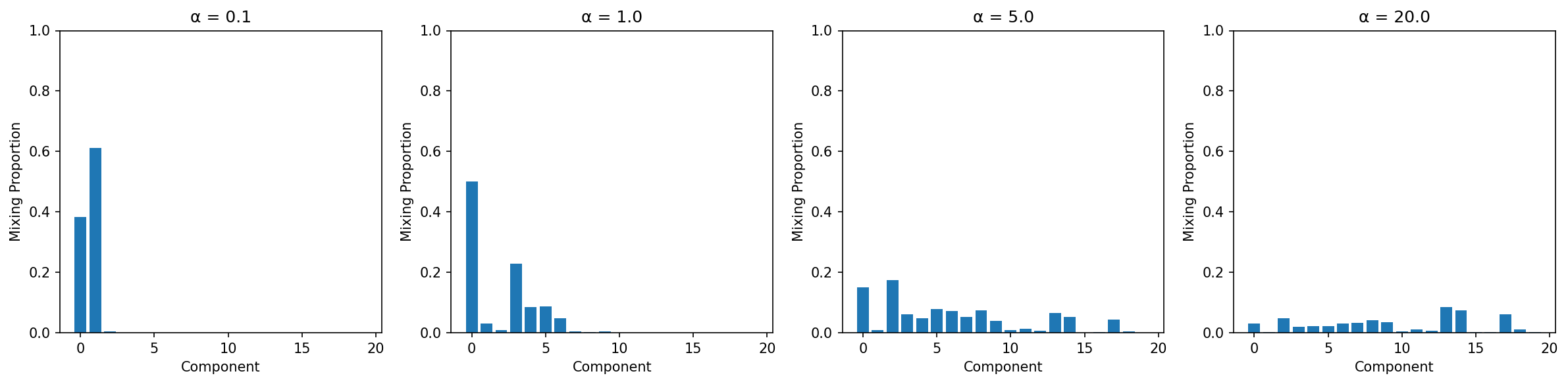
Interpretation:
- α = 0.1: First component dominates (few clusters)
- α = 1.0: Moderate spread (balanced)
- α = 5.0: More components active (many clusters)
- α = 20.0: Very even spread (diffuse)
Real-World Applications
Anomaly Detection
- Normal data forms clusters
- Outliers create singleton clusters
- α controls sensitivity to outliers
Topic Modeling
- Documents are mixtures over topics
- DPMM discovers number of topics automatically
- Each topic is a distribution over words
Genomics
- Cluster genes by expression patterns
- Number of functional groups unknown
- DPMM identifies distinct expression profiles
Image Segmentation
- Pixels cluster by color/texture
- DPMM finds natural segments
- No need to specify number of segments
Practice Problems
Problem 1: Adjusting α
Using the observed bento data from earlier, run inference with α ∈ {0.5, 2.0, 10.0}.
a) How does the number of active clusters change?
b) How does posterior uncertainty change?
Show Solution
We reuse the gibbs_sweep from earlier, just rerunning the sampler at each $\alpha$ and reporting the average number of occupied clusters (averaging over sweeps, which avoids the single-sweep noise):
| |
Output:
α =  0.5:  E[K] = 3.21
α =  2.0:  E[K] = 3.60
α = 10.0:  E[K] = 4.76
The trend is exactly as the theory predicts: a larger concentration parameter $\alpha$ makes the model spin up more clusters (some of them spurious splits of the three real groups), while a small $\alpha$ keeps it parsimonious. Note that even at $\alpha = 0.5$ the model still finds the three genuine clusters — the data are clearly separated enough that the likelihood overrides the prior’s pull toward fewer clusters.
Problem 2: Sequential Learning
Chibany receives bentos one at a time. Implement online learning where the model updates as each bento arrives.
Hint: One simple approach reuses the slice sampler you already have — after each new bento arrives, rerun the sampler on all data seen so far and report the occupied clusters. (A more efficient approach would warm-start from the previous posterior instead of restarting; that is the idea behind sequential Monte Carlo.)
Show Solution (sketch)
This is left as an implementation exercise. The structure below is pseudo-code — run_sampler is the function from Problem 1; the point is the outer loop over a growing data prefix, not a new inference algorithm:
| |
Expected behavior: the number of occupied clusters grows as genuinely new bento types first appear, then stabilizes once each type has been seen — the model commits to a new cluster only when the data force it to.
What We’ve Accomplished
We started with a mystery: bentos with an average weight that doesn’t match any individual bento. Through this tutorial, we:
- Chapter 1: Understood expected value paradoxes in mixtures
- Chapter 2: Learned continuous probability (PDFs, CDFs)
- Chapter 3: Mastered the Gaussian distribution
- Chapter 4: Performed Bayesian learning for parameters
- Chapter 5: Built Gaussian Mixture Models with EM
- Chapter 6: Extended to infinite mixtures with DPMM
You now have the tools to:
- Model complex, multimodal data
- Discover latent structure automatically
- Quantify uncertainty in clustering
- Perform Bayesian inference with GenJAX
Where this goes next
Clustering was about finding structure in a pile of data. The chapters ahead turn the same Bayesian machinery toward new questions:
- Chapter 7: Bayesian Generalization asks how you learn a concept from a handful of examples — the same posterior-over-hypotheses idea, but now the hypotheses are sets (rules), and the payoff is a model of how humans generalize.
- Chapters 8–11: the Bayesian-networks spine zoom out from a single model to the structure of models: drawing them as graphs (Bayes nets), reading off which variables inform which (conditional independence and d-separation), distinguishing seeing from doing (causal Bayes nets and the do-operator), and measuring it all in bits (information theory). The DPMM you just built is itself a Bayes net — Chapter 8 makes that explicit.
- Chapter 12: Hierarchical Bayes stacks priors on priors so the model can learn its own prior from related problems — and, as we noted above, it’s exactly the move that tames the DPMM’s cluster-count behavior.
So the mystery bentos were just the beginning: the rest of Tutorial 3 is about graphs, causes, information, and learning the prior itself.
Further Reading
Theoretical Foundations
- Ferguson (1973): “A Bayesian Analysis of Some Nonparametric Problems” (original DP paper)
- Teh et al. (2006): “Hierarchical Dirichlet Processes” (extensions to HDP)
- Austerweil, Gershman, Tenenbaum, & Griffiths (2015): “Structure and Flexibility in Bayesian Models of Cognition” (Chapter in The Oxford Handbook of Computational and Mathematical Psychology - comprehensive overview of Bayesian nonparametric approaches to cognitive modeling)
Practical Implementations
- Neal (2000): “Markov Chain Sampling Methods for Dirichlet Process Mixture Models” (MCMC inference)
- Walker (2007): “Sampling the Dirichlet Mixture Model with Slices” (the slice sampler used in this chapter)
- Kalli, Griffiths, & Walker (2011): “Slice sampling mixture models” (refinements and a clear exposition)
- Blei & Jordan (2006): “Variational Inference for Dirichlet Process Mixtures” (scalable inference)
- Stephens (2000): “Dealing with label switching in mixture models” (post-hoc relabeling for valid per-component summaries)
GenJAX Documentation
- GenJAX GitHub - Official repository
- Probabilistic Programming Examples - Gen.jl (sister project)
Key Takeaways
- DPMM: Bayesian nonparametric model that learns K automatically
- Stick-breaking: Defines mixing proportions for infinite components
- CRP: Intuitive “customers and tables” interpretation
- α: Concentration parameter controlling cluster tendency
- Slice sampler: Auxiliary slice variables $u_i$ adaptively truncate the infinite stick, so each Gibbs sweep only handles finitely many live clusters
- Label switching: Cluster labels are arbitrary — summarize with label-invariant quantities (co-clustering, posterior over $K$) or a single relabeled sample, never raw per-label averages
Interactive Exploration
Want to experiment with DPMMs yourself? Try our interactive Jupyter notebook that lets you:
- Adjust the concentration parameter α and see its effect on clustering
- Add or remove data points and watch the model adapt
- Change the truncation level K_max
- Visualize posterior distributions in real-time
Try It Yourself!
📓 Open Interactive DPMM Notebook on Google Colab
No installation required - runs directly in your browser!
The notebook includes:
- Complete DPMM implementation with stick-breaking
- Interactive widgets for all parameters
- Real-time visualization of posteriors
- Guided exercises to deepen understanding
This is a great way to build intuition for how α, K_max, and the data itself interact to produce the posterior distribution.