Continuous Concepts & Shepard's Law
On-ramp 3: continuous concepts and the rectangle game
So far every hypothesis space has been a finite list — the seven number-rules of §4–§6. That’s why we could enumerate: score every rule, normalize, done. But many real concepts live on a continuous scale. “Healthy blood-sugar level,” “a comfortable room temperature,” “roughly lunchtime” — each is an interval on some axis, and there are infinitely many candidate intervals. Does the framework still work?
It does, and almost nothing changes. Tenenbaum’s rectangle game makes this concrete: imagine the property applies to items inside some unknown interval (in 2-D, an unknown rectangle), you see a few example items known to have the property, and you must judge which other positions have it. The hypothesis space $\mathcal{H}$ is now “every interval $[\text{lo}, \text{hi}]$,” and a hypothesis’s size $|h|$ is its length, $\text{hi} - \text{lo}$. The strong-sampling likelihood is exactly what it was, with length playing the role of set-size: an interval of length $L$ makes each example $1/L$-likely, so $n$ examples are $(1/L)^n$-likely. The size principle carries over unchanged — shorter intervals fit a tight cluster of examples far better than long ones.
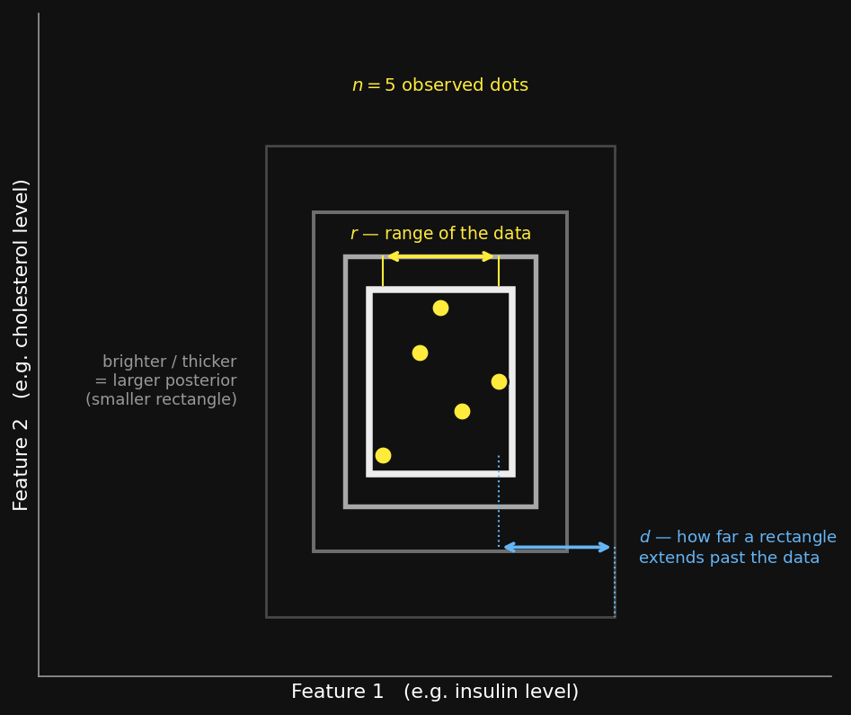
The picture above is the 2-D version (Tenenbaum, 1999): the dots are the observed examples, and every rectangle that encloses all of them is a candidate hypothesis. By the size principle, the smallest enclosing rectangles get the most posterior weight (shown brighter), so generalization concentrates near the data. Two quantities will matter when we compare to people: $r$, the range the dots span, and $d$, how far past that range a rectangle (or a person’s judgment) extends. The 1-D interval is just this with one axis instead of two, and it’s the case we’ll actually compute below.
Infinitely many hypotheses? Use a grid.
We can’t literally enumerate every real interval, but we don’t need to. We lay down a fine grid of candidate endpoints and enumerate the intervals between them — exactly the “score every hypothesis and normalize” move from §5, just over a grid instead of a hand-written list. Make the grid finer and the answer converges to the continuous one. (This is the same spirit as Chapter 2’s “area under the curve”: approximate a continuous quantity by a fine discretization.)
Building the interval learner
The code is the §5/§6 enumeration, adapted from a list of number-rules to a grid of intervals. We observe a tight cluster of examples — say at positions 9, 10, 11 — and compute what’s called the generalization gradient: for every position $y$ on the grid, the posterior-weighted vote of the intervals that contain it. (It’s the exact continuous analog of the per-number vote from §5 — the same $\sum_h \mathbf{1}[y\in h] \cdot p(h\mid X)$, now swept across a whole axis of query positions $y$.)
| |
Output:
  g(10.0) = 1.0
  g(12.0) = 0.545
  g(13.0) = 0.339
  g(15.0) = 0.15
  g(18.0) = 0.039
The gradient is flat at 1.0 across the observed cluster (every consistent interval contains positions inside the data), then decays smoothly as $y$ moves away — generalization falls off with distance, exactly the behavior Shepard measured. And it’s the same posterior-weighted vote as the number game; only $\mathcal{H}$ changed, from a list of sets to a grid of intervals.
Shepard’s law, emerging from the model
Recall the promise from §3: Shepard found generalization decays exponentially with distance, and showed analytically that a rational learner should produce that exponential. We won’t reproduce his analytic proof here; instead we’ll demonstrate computationally that the exponential falls out of our interval model — we never put it in, yet the gradient our code produces is (to a close approximation) exponential. The check needs nothing fancier than division. The signature of exponential decay is a constant ratio: each fixed step away from the data multiplies the gradient by the same factor (e.g. $e^{-1}$ per unit of distance). If instead the gradient fell off linearly or as a bell curve, that step-to-step ratio would drift. So let’s just walk outward from the edge of the data and print the ratio of each value to the previous one:
| |
Output:
distance past data | g      | ratio to previous
        1          | 0.5452 |   (first point)
        2          | 0.3387 | 0.621
        3          | 0.2230 | 0.659
        4          | 0.1503 | 0.674
        5          | 0.1009 | 0.671
        6          | 0.0656 | 0.650
Every step out multiplies the gradient by roughly the same factor (~0.65) — a near-constant ratio, which is the hallmark of exponential decay. (The small wiggle, 0.62–0.67, is a discretization artifact of our finite grid, not a departure from the exponential; a finer grid steadies it.) We never put an exponential anywhere in the model; we only assumed a hypothesis space of intervals and a strong-sampling likelihood. Shepard’s universal law emerges from Bayesian generalization over intervals. This is the computational counterpart of the promise in §3: the exponential gradient is not an assumption we baked in but a consequence of the model — here shown empirically, and provable analytically (as Shepard did) for the idealized continuous case.
One flaw, one fix: the exponential prior
There’s a catch, and it’s the same one Tenenbaum found when he compared this model to human data. With a flat prior over intervals — every interval length equally likely a priori — the model over-extends: it keeps a stubborn amount of belief on very long intervals, so its gradient decays too slowly and predicts the property too far from the data. People don’t do this; they generalize more tightly.
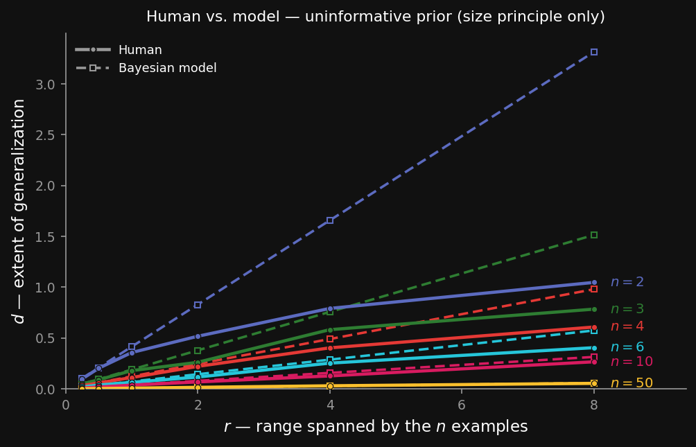
The figure above (data from Tenenbaum, 1999) plots $d$ against $r$, one curve per number of examples $n$, for people versus the flat-prior model. People’s generalization saturates — past a point, more spread doesn’t make them extend much further — but the flat-prior model keeps reaching outward. The gap between the two curves is the over-extension we need to fix.
The fix is a better prior over interval length. Long intervals should be a priori less likely than short ones, and the natural choice is the exponential distribution — our first genuinely new distribution this chapter.
The exponential distribution (define-before-use)
The exponential distribution is a probability distribution over a single non-negative number $s \ge 0$ (here, an interval’s length). Its density is
$$p(s) = \lambda e^{-\lambda s}, \qquad s \ge 0,$$
with one parameter, the rate $\lambda > 0$. Read it as: small values of $s$ are most likely, and the
density falls off — exponentially — as $s$ grows. Its mean is $1/\lambda$, so a larger rate $\lambda$ pulls
the typical value smaller (favoring shorter intervals more strongly). This is the same $e^{-(\text{something})}$
decay shape you met in §3, now serving as an honest probability distribution (it integrates to 1 over
$s \ge 0$). In code we only need its log, $\log p(s) = \log \lambda - \lambda s$; since the constant
$\log \lambda$ washes out when we normalize the posterior, the prior contributes just $-\lambda s$ — which is
exactly the -exp_rate * length line already sitting in our gradient function above.
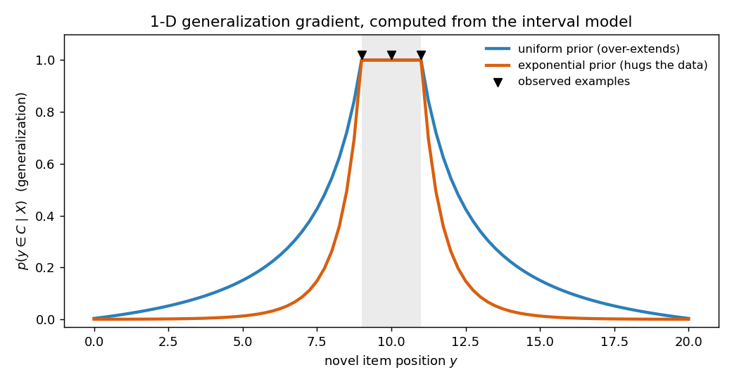
So we don’t even need new code — we just switch the prior on. Compare the flat-prior gradient with an exponential-prior one (rate $\lambda = 0.5$):
| |
Output:
       distance:   +1     +2     +4     +7
  flat  prior:  0.545  0.339  0.15   0.039
  exp   prior:  0.263  0.086  0.013  0.001
The exponential prior pulls every off-data prediction down — the gradient now hugs the data instead of over-reaching. That tighter curve is what matches human generalization. Here are the two gradients side by side, computed by our own code:
And here is the payoff against real behaviour: with the exponential prior added, the model’s $d$-vs-$r$ curves bend over and land on the human curves — the over-extension from the previous figure is gone.
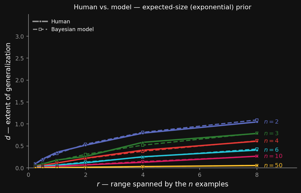
The fit is the one Tenenbaum (1999) reports: the size principle supplies the ordering (fewer examples → generalize further), and the exponential prior supplies the saturation (don’t extend without bound). Neither ingredient alone matches people; together they do.
What the rectangle game adds
Nothing in the framework changed for continuous concepts — same posterior-weighted vote, same strong-sampling size principle, computed by enumeration over a grid instead of a list. But two payoffs are new and important. First, Shepard’s exponential law emerges from the model rather than being assumed — the gradient our code produces decays by a near-constant factor at each step away from the data, the signature of exponential decay (shown here computationally, and provable analytically for the idealized case). Second, the prior matters: a flat prior over-extends, and an exponential prior on size pulls generalization in to match people. Holding that thought — the prior is doing real work — sets up the last question of the chapter: where does the hypothesis space (and its prior) come from, and what if we choose it badly? That’s No Free Lunch.