The Number Game & the Size Principle

Generalization is a posterior-weighted vote

Now the payoff. We can state, in one line, how to predict whether a novel item $y$ has the property. The probability is the total posterior belief sitting on the hypotheses that contain $y$:

$$p(y \in C \mid X) = \sum_{h \in \mathcal{H}} \mathbf{1}[y \in h] \cdot p(h \mid X).$$

Read it in plain words first: every hypothesis casts a vote. Each one’s vote is weighted by how much we now believe it — its posterior $p(h \mid X)$ — and a hypothesis votes “yes” for $y$ only if it actually contains $y$ (that’s the $\mathbf{1}[y \in h]$). Sum the yes-votes and you have the prediction. This is the two-rule calculation from §2, written for any number of rules. Every symbol in it was defined in §4.

Computing the vote by enumeration

Here is the one genuinely new code idea in this section — and it makes things simpler, not harder. Because $\mathcal{H}$ is a finite list, we don’t need to sample anything: we can score every hypothesis directly and normalize. That’s it. (The vmap-over-rows you just met in §4 is exactly the tool for “score every hypothesis at once.”)

For this section we keep the weak-sampling likelihood from §2: a rule is consistent with the data if it contains every observed example (likelihood 1), and impossible if it misses any (likelihood 0). That’s enough to make the vote work; in §6 we’ll meet a sharper likelihood — strong sampling — that also prefers smaller rules among the consistent ones.

Suppose you’re told that 10 has the property, and you want to predict which other numbers do. First, the posterior over rules:

 1
 2
 3
 4
 5
 6
 7
 8
 9
10
11
12
13
14
15
16
17
18

import jax.numpy as jnp
# (H and prior are the hypothesis matrix and uniform prior defined earlier in §4.)

# We observed that the number 10 has the property. 10 lives in COLUMN 9 (number n -> column n-1).
observed = 9    # column index for the number 10

# Likelihood: a rule is consistent (1) if it contains the observed number, else impossible (0).
# H[:, observed] reads DOWN column `observed` -- it picks that number's 0/1 membership from
# every rule at once (the ":" means "all rows"; rows are RULES now, so this is one entry per
# rule -- not one entry per data sample, the way columns worked back in the GenJAX tutorial).
consistent = H[:, observed]

# Posterior over rules: prior x likelihood, then normalize. (Bayes' rule, scored per rule.)
post = prior * consistent
post = post / post.sum()

for label, p in zip(labels, post):
    print(f"  P({label:16s} | saw 10) = {round(float(p), 3)}")

Output:

  P(all numbers      | saw 10) = 0.25
  P(even numbers     | saw 10) = 0.25
  P(multiples of 3   | saw 10) = 0.0
  P(multiples of 10  | saw 10) = 0.25
  P(powers of 2      | saw 10) = 0.0
  P(numbers 1-10     | saw 10) = 0.25
  P(numbers 20-30    | saw 10) = 0.0

Four rules survive — “all numbers,” “even numbers,” “multiples of 10,” and “numbers 1–10” all contain 10 — and with a uniform prior they split the belief evenly, 0.25 each (the other three are ruled out, so the four survivors renormalize from 1/7 up to 1/4). “Multiples of 3,” “powers of 2,” and “numbers 20–30” don’t contain 10, so observing it is impossible under them. (Notice the surviving rules are still tied — weak sampling can’t yet tell the tight “multiples of 10” from the loose “all numbers.” §6 fixes that.)

Now the vote. For each number $y$, we sum the posterior of the rules that contain it — that’s the chapter equation, computed one number at a time:

1
2
3
4
5
6
7
8
9

import jax.numpy as jnp
# (continued: H and post come from the cell just above.)

# Predict P(number n has the property | data) for every number 1..30.
predictive = jnp.array([jnp.sum(post * H[:, n - 1]) for n in numbers])

# Show a few:
for n in [10, 2, 5, 7, 25]:
    print(f"  P({n:2d} has the property | saw 10) = {round(float(predictive[n - 1]), 3)}")

Output:

  P(10 has the property | saw 10) = 1.0
  P( 2 has the property | saw 10) = 0.75
  P( 5 has the property | saw 10) = 0.5
  P( 7 has the property | saw 10) = 0.5
  P(25 has the property | saw 10) = 0.25

Read the gradient off the numbers. 10 itself scores 1.0 — every surviving rule contains it. 2 scores 0.75: it’s in “even numbers” and “numbers 1–10” and “all numbers” — three of the four surviving rules, each worth 0.25. 5 and 7 each score 0.5 — both sit in “numbers 1–10” and “all numbers” (two of the four survivors). 25 scores 0.25 — the only surviving rule that reaches it is the catch-all “all numbers” (it’s too big for “numbers 1–10” and isn’t even). That floor of 0.25 is the catch-all’s signature: it contains every number, so no number ever drops to zero while it survives. From a single example, generalization is broad and graded: lots of numbers get moderate support, with no sharp rule yet. That diffuse spread is exactly the human pattern after one example. (We’ll picture this gradient — and watch it sharpen into a rule — in §6, once the size principle is switched on.)

Where did the examples come from? Weak vs. strong sampling

Look again at the likelihood we used in §5: a rule was consistent (likelihood 1) if it contained the data, impossible (likelihood 0) otherwise. That rule is blind to size — “multiples of 10” and “all numbers” both contain 10, so both got likelihood 1, and they ended up tied. But intuitively a tight rule that barely fits the data should be favored over a loose one that fits it only incidentally. To get there we have to think about a question we’ve so far skipped: how were the observed examples generated in the first place?

There are two natural answers, and they give two different likelihoods.

• Weak sampling. The examples came from somewhere outside the rule — the world handed them to you — and you merely checked whether each one happens to fall in $h$. Under this story the likelihood is exactly the size-blind one from §5: $$p(X \mid h) = \begin{cases} 1 & \text{if every } x_i \in h \\ 0 & \text{otherwise} \end{cases}$$ A rule either contains the data or it doesn’t; its size never enters.

• Strong sampling. The examples were drawn from inside the rule — as if someone reached into the set $h$ and pulled out members at random. If $h$ has $|h|$ members and each example is an independent uniform draw from it, then each draw has probability $1/|h|$, and $n$ independent draws have probability $$p(X \mid h) = \left(\frac{1}{|h|}\right)^{!n}.$$ Now size matters enormously: a small rule assigns high probability to any particular member, because there are few members to choose from.

(Recall $|h|$ from §4 — the size of a rule, the number of 1s in its row, which we computed for every rule with jax.vmap(jnp.sum)(H). And $n$ is just the number of observed examples, the same $n$ you’ve used since Chapter 4.)

The size principle

That little exponent $(1/|h|)^n$ is the whole game. Under strong sampling, smaller hypotheses get higher likelihood — and the advantage grows exponentially with the number of examples $n$. This is the size principle: among the rules consistent with your data, the data votes hardest for the smallest one, and ever more decisively as you see more examples.

The intuition has a name: the suspicious coincidence. Suppose you see the numbers $\{10, 20, 30\}$. They’re all multiples of 10 — but they’re also all even numbers. If the true rule were “even numbers,” it would be a suspicious coincidence that all three happened to land on multiples of 10: among our numbers 1–30 there are 15 even numbers and only 3 of them are multiples of 10, so picking three multiples of 10 by chance from “even numbers” is a long shot. Strong sampling formalizes that suspicion: “even numbers” could have produced this data, but it would have been lucky to. “Multiples of 10” predicts exactly this kind of data — it has only three members and all three showed up — so it wins.

Strong sampling on the number game

Let’s watch the size principle reshape §5’s result. Recall that observing 10 left four rules tied — the tight “multiples of 10” (size 3) was no better than the loose catch-all “all numbers” (size 30). Strong sampling breaks that tie, and it breaks it harder with every new example.

The new code is one function, log_likelihood, with the two sampling stories built in. We work in log space, using the fact that logs turn products into sums: $\log(ab) = \log a + \log b$. The likelihood of several independent examples is a product of per-example probabilities, so in log space it becomes a sum — which is why the function below just adds up per-example log-probabilities with .sum(). We bother with logs because $(1/|h|)^n$ can get very small, and summing logs is the numerically safe way to multiply many tiny numbers. The final step — jnp.exp(... - max), then divide by the sum — is exactly the importance-weight normalization you ran in the GenJAX tutorial; the only new thing is that we enter log space by hand with jnp.log rather than receiving log-weights back from generate.

 1
 2
 3
 4
 5
 6
 7
 8
 9
10
11
12
13
14
15
16
17
18
19
20
21
22
23
24
25
26
27
28
29
30
31
32
33
34
35
36
37
38
39
40
41
42
43
44
45
46
47
48
49
50
51
52
53
54
55
56
57

import jax
import jax.numpy as jnp
# (H, prior, labels, numbers are from §4: the 7-rule number game and the uniform prior.)

def log_likelihood(rule, observed, strong):
    """log p(X | rule) for one rule, under weak or strong sampling.

    `observed` is a jnp.array of observed COLUMN indices; `strong` is a plain Python bool.
    """
    # rule[observed] indexes the rule by an ARRAY of positions, returning one entry per
    # observed number at once -- e.g. rule[jnp.array([9, 19])] gives [rule[9], rule[19]].
    # Each entry is 1.0 if the rule contains that observed number, else 0.0.
    # (JAX wants a jnp.array here, not a plain Python list -- see how `observed` is built below.)
    in_rule = rule[observed]
    size = rule.sum()                 # |h|, the number of numbers this rule includes

    # We work in LOG space: take the log of each probability, so multiplying probabilities
    # becomes adding logs (the .sum() at the end). jnp.where does its FAMILIAR job from
    # Chapter 5 -- pick a value per element:
    #   strong: an in-rule example contributes log(1/size) = -log(size);
    #   weak:   an in-rule example contributes log(1)      = 0.
    # A MISSED example contributes -jnp.inf, which is log(0): "impossible under this rule,"
    # driving its whole likelihood to exactly 0 once we exponentiate at the end.
    per_example_strong = jnp.where(in_rule > 0, -jnp.log(size), -jnp.inf)
    per_example_weak   = jnp.where(in_rule > 0, 0.0,            -jnp.inf)

    # The genuinely NEW idiom: a plain Python `if` on `strong` switches the whole FORMULA.
    # `strong` is an ordinary Python True/False, fixed before any array math, so a normal
    # `if` just chooses which formula to build. (Contrast jnp.where above, which decides
    # element-by-element *inside* the array math. Rule of thumb: a plain `if` to pick a whole
    # formula from a Python flag; jnp.where to pick a value per array element.)
    per_example = per_example_strong if strong else per_example_weak

    return per_example.sum()          # sum of logs = log of the product of per-example probabilities

def posterior(observed, strong):
    """Posterior over all rules, by enumeration, under the chosen sampling story."""
    log_post = jnp.log(prior) + jax.vmap(lambda r: log_likelihood(r, observed, strong))(H)
    log_post = log_post - log_post.max()      # subtract the max for numerical stability
    p = jnp.exp(log_post)
    return p / p.sum()

# Column indices for the numbers we observe (number n -> column n-1).
one_example  = jnp.array([9])             # {10}
three_example = jnp.array([9, 19, 29])    # {10, 20, 30}

print("STRONG, after {10}:")
for label, p in zip(labels, posterior(one_example, strong=True)):
    print(f"   {label:16s} {round(float(p), 3)}")

print("STRONG, after {10, 20, 30}:")
for label, p in zip(labels, posterior(three_example, strong=True)):
    print(f"   {label:16s} {round(float(p), 3)}")

print("WEAK, after {10, 20, 30}:")
for label, p in zip(labels, posterior(three_example, strong=False)):
    print(f"   {label:16s} {round(float(p), 3)}")

Output:

STRONG, after {10}:
   all numbers      0.062
   even numbers     0.125
   multiples of 3   0.0
   multiples of 10  0.625
   powers of 2      0.0
   numbers 1-10     0.188
   numbers 20-30    0.0
STRONG, after {10, 20, 30}:
   all numbers      0.001
   even numbers     0.008
   multiples of 3   0.0
   multiples of 10  0.991
   powers of 2      0.0
   numbers 1-10     0.0
   numbers 20-30    0.0
WEAK, after {10, 20, 30}:
   all numbers      0.333
   even numbers     0.333
   multiples of 3   0.0
   multiples of 10  0.333
   powers of 2      0.0
   numbers 1-10     0.0
   numbers 20-30    0.0

There it is — the famous number-game effect, quantified. With one example (10), strong sampling already tilts toward the tight rule — “multiples of 10” gets 0.625, because each example is $1/3$-likely under it but only $1/30$-likely under “all numbers” — yet “even numbers” (0.125) and “numbers 1–10” (0.188) keep real mass, so generalization stays broad and graded. With three examples (10, 20, 30), the size advantage is now cubed: $(1/3)^3$ vs $(1/30)^3$ is a 1000-to-1 likelihood ratio, and “multiples of 10” rockets to 0.99 while everything else collapses — generalization snaps to a rule. That switch from graded similarity to a confident rule, off just three examples, is exactly what people do.

The two posteriors, side by side:

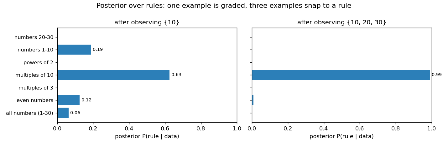
And weak sampling, for contrast: the three rules that contain all of {10, 20, 30} — “all numbers,” “even numbers,” “multiples of 10” — stay tied at 0.333 forever, no matter how many multiples of 10 you pile up. Weak sampling is size-blind, so it never notices the suspicious coincidence. That gap between the weak result (stuck at a three-way tie) and the strong result (0.99 on the tight rule) is the size principle.

Now turn the posterior back into a prediction over numbers — the posterior-weighted vote from §5, run under strong sampling for both the one-example and three-example posteriors:

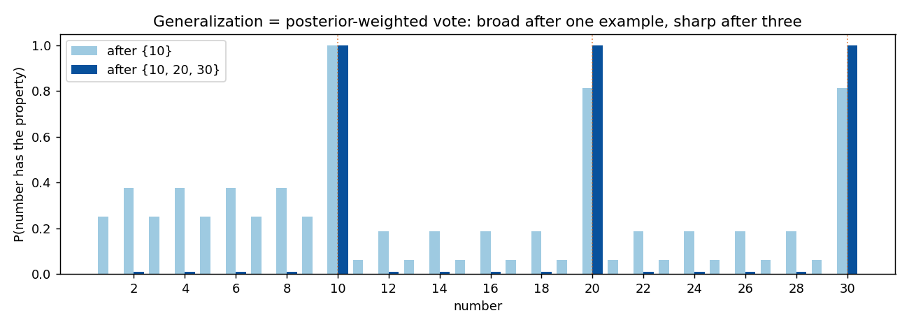
After one example the prediction already leans hard toward the multiples of 10 (20 and 30 near 0.81) while keeping a low, broad skirt over the even numbers — graded, but with the tight rule already winning. After three examples it collapses to three sharp spikes. The model didn’t switch strategies — it ran the same posterior-weighted vote both times. All that changed was how decisively the size principle concentrated the posterior, and the generalization gradient followed.

What we just reproduced: the number game

What we computed above is Tenenbaum’s number game, one of the most-studied effects in human concept learning — and worth pausing on, because you can feel it in your own head. The game: someone has a hidden rule that picks out some numbers, shows you a few that fit, and you judge which others fit.

• You’re told 10 fits the rule. Which other numbers fit? Most people feel unsure — 20? 5? 30? lots seem plausible. The guess is broad and fuzzy. (Our model after {10}: a wide, graded gradient.)
• Now you’re told 10, 20, and 30 all fit. Now which fit? Almost everyone snaps to a crisp rule — “multiples of 10”: 40 yes, 25 no. (Our model after {10, 20, 30}: a sharp spike on the multiples of 10.)

The same first example, 10, leads to completely different generalization depending on what follows it — and our model reproduced both regimes with no change of strategy, just the size principle concentrating the posterior as evidence accumulated. That is the whole point: one mechanism produces both similarity-like (graded) and rule-like (all-or-none) generalization, and switches between them automatically as the data warrants.