Setup & the Framework

What you’re bringing with you

This chapter changes exactly one thing about what you already know — and it is worth saying up front what stays the same, because almost everything does.

The golden sticker

Chibany has been receiving bentos for months, and lately they have noticed something odd. Some bentos arrive with a tiny golden sticker on the side. Others don’t.

Chibany has no idea what the sticker means. Maybe it marks the day of the week the bento was made. Maybe it marks a particular chef. Maybe it’s a price tier, or a loyalty reward, or something else entirely. All Chibany gets to see is which bentos have the sticker and which don’t.

Being a probabilist, Chibany decides to figure it out the only way they can: by guessing rules and watching which guesses survive. They write down every plausible rule the sticker might follow —

“only on Mondays” “only tonkatsu bentos” “only bentos heavier than 400 g” “every bento” (maybe the sticker means nothing at all)

— and then they wait. As more sticker’d bentos arrive, some rules will keep fitting and others will be ruled out or made to look unlikely. Whatever rules are still standing after the data is what Chibany should believe.

That is the entire idea of this chapter, and it already contains its three moving parts:

• The golden sticker is a novel property — something we want to predict for new bentos.
• Each rule is a hypothesis: and notice that a rule is really just a set of bentos — “only Mondays” is the set of all Monday bentos, “every bento” is the set of all of them.
• The rules still standing after Chibany sees some data form a posterior over hypotheses.

The question Chibany actually wants to answer is a prediction: I see one bento with a golden sticker — should I expect the next one to have it too? We will build up to answering exactly that.

From “which event?” to “which set?”

Before we write down any general framework, let’s cross the one genuinely new idea on the smallest possible example — because the leap from “the unknown is a yes/no fact” to “the unknown is a set” is the only thing here you haven’t done before.

Start with something you’ve already solved

Recall the taxicab problem from the GenJAX tutorial (Chapter 4). A taxi was involved in an accident at night. The unknown was a single yes/no fact: was the taxi blue or green? In that chapter we wrote the hypothesis with a capital $H$; here we’ll use a lowercase $h$ for one hypothesis (one candidate answer), because in a moment we’ll have a whole list of them — $h_1, h_2, \dots$ — and want a clean symbol for a single member. So, two competing possibilities,

$$h \in \{\text{blue},\ \text{green}\}.$$

and Bayes’ rule ranked them: a prior over the two colors, a likelihood for the witness’s report, and a posterior that combined them. Two hypotheses, and we asked which one the data favored.

“Blue” was a set all along

Here is the small reframing that opens up the whole chapter. When we said the taxi was “blue,” what we really meant was that it belonged to the set of all blue taxis. “Green” is the set of all green taxis. An event — in the sense you learned in the very first tutorial — is just a subset of the possible outcomes. So the hypotheses in the taxicab problem were sets the entire time. We simply never needed to look at them that way, because the two sets didn’t overlap and we only cared which one the taxi fell into.

What’s new: overlapping sets of different sizes

Generalization is what happens when we take that same “which set?” question and let the sets get interesting:

• the candidate sets can overlap — a single bento can satisfy “only Mondays” and “every bento” at once, so one item can belong to many hypotheses; and
• the candidate sets can differ in size — “only tonkatsu bentos” is a small, specific set, while “every bento” is the largest set possible.

That’s the only genuinely new wrinkle. Once hypotheses are sets that overlap and vary in size, “which set does the property follow?” becomes a much richer question than “blue or green?” — but it is answered with the exact same Bayes’ rule.

A two-rule example you can hold in your head

Let’s make it concrete with just two rules, so the whole posterior fits on one line. Chibany lines up a tiny menu of four bentos and numbers them by weight, lightest to heaviest — so bento 0 is the lightest, bento 3 the heaviest. Two candidate rules for the golden sticker are on the table:

• Rule A — “the two lightest bentos”: the set $\{0, 1\}$.
• Rule B — “the lighter half”: the set $\{0, 1, 2\}$.

Both rules contain bento 0 and bento 1; they differ only on bento 2 (in B, not in A) and agree that bento 3 (the heaviest) is out. Suppose Chibany starts with no reason to prefer either rule — a flat (uniform) prior, $p(A) = p(B) = 0.5$ — and then observes one sticker’d bento: bento 1.

Before we can update, we need a likelihood — a rule for how probable the observation is under each hypothesis. We’ll use the simplest one, called weak sampling:

Apply it here: bento 1 is in both Rule A and Rule B, so under weak sampling both have likelihood 1 — neither is ruled out. Posterior ∝ likelihood × prior, so each rule’s posterior is $1 \times 0.5 = 0.5$ (then normalized), and the belief stays split evenly:

$$p(A \mid \text{bento 1 has the sticker}) = p(B \mid \dots) = 0.5.$$

Now Chibany can answer the prediction they actually care about. Is the next bento — say, bento 2 — likely to have the sticker? Bento 2 is in Rule B but not in Rule A. So only the rules that contain bento 2 vote “yes,” weighted by how much we now believe each rule:

$$p(\text{bento 2 has the sticker} \mid \text{data}) = \underbrace{p(B \mid \text{data})}_{\text{B contains 2}} = 0.5.$$

Bento 0, by contrast, is in both surviving rules, so its predicted probability is $p(A) + p(B) = 1.0$ — we’re certain. And bento 3 is in neither, so its predicted probability is $0$.

You have just done Bayesian generalization. The prediction for a new item is the total belief sitting on the rules that contain it. Everything else in this chapter — bigger rule-sets, the “suspicious coincidence” that makes smaller rules win, continuous rules — is this same calculation at larger scale.

The same thing in code

Because there are only two hypotheses, we can do something even simpler than the taxicab’s sampling: we can write down both rules, score each one by prior × likelihood (exactly Bayes’ rule), and normalize. With a handful of hypotheses there is no need to sample at all — we just check every rule directly. (Later in the chapter, when the rules number in the dozens, this same “score every rule and normalize” idea is all we’ll need.)

We represent each rule as a row of 0s and 1s — a membership list, the same 0/1 “is it in the set?” idea you used to describe an event in the first tutorial:

 1
 2
 3
 4
 5
 6
 7
 8
 9
10
11
12
13
14
15
16
17
18
19
20
21
22
23
24
25
26
27
28
29
30
31
32
33
34
35

import jax.numpy as jnp

# A tiny menu of 4 bentos (columns 0-3). Two candidate rules (rows).
# A 1 means "this bento is in the rule"; a 0 means it is not.
rule_A = jnp.array([1.0, 1.0, 0.0, 0.0])   # Rule A = {0, 1}     ("the two lightest bentos")
rule_B = jnp.array([1.0, 1.0, 1.0, 0.0])   # Rule B = {0, 1, 2}  ("the lighter half")

# Flat (uniform) prior: each rule starts at probability 0.5.
prior_A = 0.5
prior_B = 0.5

# --- We observed that bento 1 has the sticker. ---
# A rule can only "explain" a sticker'd bento if that bento is in the rule. So the
# likelihood of "bento 1 has the sticker" under a rule is 1 if the rule contains bento 1,
# and 0 if it doesn't. We read that straight off the membership list at position 1.
likelihood_A = rule_A[1]    # is bento 1 in Rule A?  -> 1.0
likelihood_B = rule_B[1]    # is bento 1 in Rule B?  -> 1.0

# Bayes' rule: posterior is proportional to prior x likelihood. Then normalize so the
# two posteriors add to 1.
unnormalized_A = prior_A * likelihood_A
unnormalized_B = prior_B * likelihood_B
total = unnormalized_A + unnormalized_B
post_A = unnormalized_A / total
post_B = unnormalized_B / total

print("posterior:  Rule A =", float(post_A), " Rule B =", float(post_B))   # 0.5, 0.5
# (float() unwraps each JAX scalar so it prints as a plain 0.5 instead of Array(0.5, ...),
#  the same de-cluttering trick you saw with int() back in the GenJAX tutorial.)

# Predict: does the sticker generalize to a given bento? Add up the posterior of every
# rule that CONTAINS that bento -- "the total belief sitting on the rules that contain it."
for bento in range(4):
    p = post_A * rule_A[bento] + post_B * rule_B[bento]
    print(f"  predicted P(sticker) for bento {bento} = {float(p)}")

Output:

posterior:  Rule A = 0.5  Rule B = 0.5
  predicted P(sticker) for bento 0 = 1.0
  predicted P(sticker) for bento 1 = 1.0
  predicted P(sticker) for bento 2 = 0.5
  predicted P(sticker) for bento 3 = 0.0

The printed predictions match what we worked out by hand: bento 0 is certain (in both rules), bento 2 is a coin flip (in one rule), bento 3 is impossible (in neither). Every line of that code is Bayes’ rule and a membership lookup — no new machinery, just the rules written as 0/1 lists.

A target to aim for: Shepard’s law

Before we scale the two-rule example up into a general method, it helps to know what a good method should produce. There is a striking empirical fact about how people (and animals) generalize, and any model worth its salt should reproduce it.

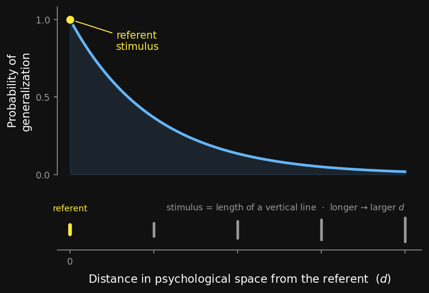
In a classic 1987 paper, Roger Shepard (Shepard, 1987) measured how willing people are to extend a property from one stimulus to another as the two stimuli grow more different. The pattern was remarkably consistent across senses and species: the probability of generalizing falls off smoothly as the two stimuli get further apart, and it falls off at a particular rate — an exponential one. Writing $d$ for the distance between two stimuli, then in suitable units

$$g(d) = e^{-d},$$

where $g$ is the probability of generalizing. (More generally the rate can differ, $g(d) = e^{-d/\tau}$ for some scale $\tau$; we set $\tau = 1$ here to keep the picture simple.) Here $e^{-d}$ is just a curve that starts at 1 when $d = 0$ (no distance, certain to generalize) and decays smoothly toward 0 as $d$ grows — you’ve seen the $\exp(-\ldots)$ form before, inside the Gaussian bell curve in Chapter 3, where it likewise equals 1 at the center and decays to zero (the Gaussian’s is a bell, Shepard’s is a sharper cusp — same “exponential of a negative quantity,” different curve). We will meet $e^{-\lambda s}$ as a full probability distribution — the exponential distribution — later in the chapter, in §8; for now it is only a curve.

Shepard’s law is descriptive: it tells us generalization decays exponentially, but not why. That “why” is exactly what the framework we’re about to build delivers. By §8 we will not assume the exponential — we will watch it emerge from the model, falling out of the posterior-weighted vote you already met (and, as Shepard first showed, it can be proved analytically for the idealized case). Keep $g(d) = e^{-d}$ in the back of your mind as the target.

The framework, named

We now have everything we need to state the method in general — and because §2 already made “a hypothesis is a set” concrete on two rules, none of the symbols below should feel abstract. Each one is something you have already used, pointed at a slightly new object. The framework in this form — generalization as Bayesian inference over a hypothesis space of consequential sets, unifying Shepard’s law with similarity- and rule-based generalization — is due to Tenenbaum & Griffiths (2001), building on Shepard’s normative account.

Notation lock-in

We will use five symbols throughout the rest of the chapter. Take a moment with them now; each is defined here before it appears in any formula.

• $h$ — a single hypothesis: one candidate rule, i.e. one set of items. (In the taxicab problem this was “blue” or “green”; now it can overlap other hypotheses and vary in size, as in §2.)
• $\mathcal{H}$ — the hypothesis space: the whole list of candidate hypotheses under consideration. (The script letter $\mathcal{H}$ is new notation; read it as “the collection of all the $h$’s.”)
• $X = \{x_1, \dots, x_n\}$ — the observed examples: the $n$ items we’ve seen to have the property (the sticker’d bentos; the example numbers in the number game below).
• $y$ — a novel item we want to judge: does it have the property?
• $C$ — the true (unknown) set the property actually picks out. This is not one of our $h$’s — it is the truth our hypotheses are guesses at. Our whole goal is to predict the event “$y \in C$” (is $y$ really in the true set?) from the examples $X$.

The three ingredients — exactly Bayes’ rule, new object

These are the same three pieces from Chapter 4, now applied to hypotheses that are sets:

• Prior $p(h)$ — how plausible each rule is before seeing data.
• Likelihood $p(X \mid h)$ — how probable the observed examples are if $h$ were the true rule.
• Posterior $p(h \mid X) \propto p(X \mid h) p(h)$ — our updated belief in each rule after the data. Identical in form to every Bayesian update you’ve done; only the meaning of $h$ has changed.

The indicator: a compact way to ask “is $y$ in $h$?”

One more symbol, and it is one you have almost seen. To write the prediction rule compactly we need a way to say “1 if $y$ is in the set $h$, and 0 otherwise.” We write that as

$$\mathbf{1}[y \in h] = \begin{cases} 1 & \text{if } y \in h \\ 0 & \text{if } y \notin h \end{cases}$$

This indicator is nothing new in substance: it is exactly the 0/1 membership you already used to write a rule as a row of 0s and 1s in §2. If $h$ is a row of the membership matrix, then $\mathbf{1}[y \in h]$ is simply the entry in column $y$ of that row. We give it a symbol only so the prediction formula in §5 fits on one line.

The hypothesis space in code

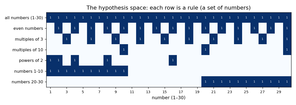
Let’s build a real, slightly bigger hypothesis space and use it for the rest of the chapter. We’ll play Tenenbaum’s number game: someone has a hidden rule that picks out some of the numbers from 1 to 30, you see a few example numbers that fit it, and you judge which other numbers fit. (We use 1–30 rather than the classic 1–100 so the whole space fits in one picture.) Each hypothesis is a rule about which numbers share the property — written, just like the two rules in §2, as a row of 0s and 1s over the numbers 1–30.

We’ll consider a small, mixed set of seven candidate rules: a few “multiples of $k$,” “powers of 2,” two magnitude intervals, and the catch-all “all numbers.” Rather than type out 7 × 30 ones and zeros by hand, we build each row from its defining test:

 1
 2
 3
 4
 5
 6
 7
 8
 9
10
11
12
13
14
15
16
17
18
19
20
21
22
23
24
25

import jax
import jax.numpy as jnp

numbers = list(range(1, 31))     # the universe: 1, 2, ..., 30 (these are the COLUMNS)

def make_rule(test):
    """Turn a yes/no test into a membership row: 1 where the test holds, else 0."""
    return jnp.array([1.0 if test(n) else 0.0 for n in numbers])

# Each ROW is one hypothesis (a rule); each COLUMN is one number (1..30, left to right).
labels = ["all numbers", "even numbers", "multiples of 3", "multiples of 10",
          "powers of 2", "numbers 1-10", "numbers 20-30"]
H = jnp.stack([
    make_rule(lambda n: True),                  # h0: all numbers   (catch-all, size 30)
    make_rule(lambda n: n % 2 == 0),            # h1: even numbers              (size 15)
    make_rule(lambda n: n % 3 == 0),            # h2: multiples of 3            (size 10)
    make_rule(lambda n: n % 10 == 0),           # h3: multiples of 10           (size 3)
    make_rule(lambda n: n in (1, 2, 4, 8, 16)), # h4: powers of 2               (size 5)
    make_rule(lambda n: 1 <= n <= 10),          # h5: an interval, numbers 1-10 (size 10)
    make_rule(lambda n: 20 <= n <= 30),         # h6: an interval, numbers 20-30(size 11)
])

# A uniform prior: before any data, every rule is equally plausible.
# H.shape is (rows, columns) = (7 rules, 30 numbers), so H.shape[0] is the number of rules.
prior = jnp.ones(H.shape[0]) / H.shape[0]    # 7 hypotheses -> each starts at ~0.143

This matrix H is the whole hypothesis space $\mathcal{H}$ — seven rules over thirty numbers — stacked into rows. Rule h0 is a catch-all — “all numbers,” the hypothesis that every number has the property. Because it contains everything, no observation can ever rule it out; it is always left standing. Including it is deliberate, and we’ll see in §6 and §9 why it matters.

We can see the whole space at a glance — each row a rule, each lit cell a number that rule includes:

 1
 2
 3
 4
 5
 6
 7
 8
 9
10
11
12

import jax
import jax.numpy as jnp
# (H is the hypothesis matrix defined just above.)

# |h| = how many numbers each rule includes. vmap runs jnp.sum once per ROW of H.
# We pass jnp.sum itself as the per-row function -- the same slot where, in earlier
# chapters, you wrote your own function like run_one_day. vmap always works the same way:
# it peels off the first axis and runs the function on each slice. Before, that first axis
# indexed random keys; here it indexes the rows of H.
sizes = jax.vmap(jnp.sum)(H)
for label, size in zip(labels, sizes):
    print(f"|h| for {label:16s} = {int(size)}")

|h| for all numbers      = 30
|h| for even numbers     = 15
|h| for multiples of 3   = 10
|h| for multiples of 10  = 3
|h| for powers of 2      = 5
|h| for numbers 1-10     = 10
|h| for numbers 20-30    = 11