Partial Pooling & Shrinkage

Partial pooling and shrinkage

Now suppose the six students share a common population prior $\text{Beta}(a, b)$ — say $\text{Beta}(6, 4)$, encoding “the typical student is about 60% tonkatsu ($\tfrac{6}{6+4} = 0.6$), with a prior strength of $a + b = 10$ bentos.” Each student’s estimate becomes their own Beta-Binomial posterior mean, $(a + k_i) / (a + b + n_i)$:

 1
 2
 3
 4
 5
 6
 7
 8
 9
10
11
12
13
14
15

import jax.numpy as jnp

names = ["Alyssa", "Ben", "Carmen", "Diego", "Emi", "Farid"]
k = jnp.array([70, 28, 6, 3, 2, 0])
n = jnp.array([100, 40, 10, 5, 2, 1])

a, b = 6.0, 4.0                       # shared population prior: mean 0.6, strength 10
population_mean = a / (a + b)

raw = k / n
posterior_mean = (a + k) / (a + b + n)   # Beta-Binomial posterior mean per student

print(f"population mean = {population_mean:.2f}\n")
for name, r, pm in zip(names, raw, posterior_mean):
    print(f"  {name:7s} raw {float(r):.2f} -> pooled {float(pm):.3f}  (shift {float(pm - r):+.3f})")

Output:

population mean = 0.60

  Alyssa  raw 0.70 -> pooled 0.691  (shift -0.009)
  Ben     raw 0.70 -> pooled 0.680  (shift -0.020)
  Carmen  raw 0.60 -> pooled 0.600  (shift +0.000)
  Diego   raw 0.60 -> pooled 0.600  (shift +0.000)
  Emi     raw 1.00 -> pooled 0.667  (shift -0.333)
  Farid   raw 0.00 -> pooled 0.545  (shift +0.545)

Read the shifts and the whole idea is there:

• Alyssa (70/100) barely moves — 0.70 → 0.691. With 100 bentos, their own data dominates the shared prior.
• Emi (2/2) and Farid (0/1) move the most — and in opposite directions: Emi crashes down from the absurd 1.00 (to 0.667) while Farid is pulled up from the absurd 0.00 (to 0.545), both toward the population. With almost no data, they lean almost entirely on the group, wherever they started.
• Carmen and Diego sit exactly at the population mean already (0.60), so they don’t move at all — pooling pulls you toward the group only to the extent you disagree with it.

This pull-toward-the-group is called shrinkage, and it is the signature behavior of a hierarchical model: estimates with little data are shrunk hardest toward the shared prior; estimates with lots of data are left almost alone. The model borrows strength across students automatically — no rule had to say “trust Emi less,” it falls out of $(a + k)/(a + b + n)$.

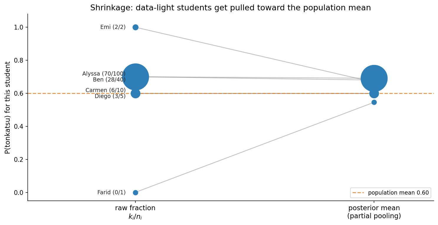
The figure makes the dependence on data size visual: marker size grows with $n_i$, and the small markers (little data) travel the farthest toward the population line, while the big markers stay put.

The hierarchical generative process

What we just computed by formula has a generative story — a recipe for how the data could have been produced — and writing it down is what makes it a hierarchical model. There are three levels:

1. A population prior $\text{Beta}(a, b)$ sits at the top.
2. Each student draws their own rate from it: $\theta_i \sim \text{Beta}(a, b)$.
3. Each student’s bentos are tonkatsu-or-not at that rate: $k_i \sim \text{Binomial}(n_i, \theta_i)$.

In symbols, the three-level hierarchy is:

$$(a, b) \sim \text{prior}, \qquad \theta_i \mid a, b \sim \text{Beta}(a, b), \qquad k_i \mid \theta_i \sim \text{Binomial}(n_i, \theta_i).$$

The dependence structure — who is drawn from whom — is a picture of arrows. The shared $(a, b)$ feeds every student’s $\theta_i$, and each $\theta_i$ feeds that student’s count $k_i$:

graph TB
    AB(("(a, b)<br/>population<br/>prior")) --> T1(("θ₁<br/>Alyssa's<br/>rate"))
    AB --> T2(("θ₂<br/>Ben's<br/>rate"))
    AB --> Td(("…"))
    AB --> TJ(("θⱼ<br/>student j's<br/>rate"))
    T1 --> K1(("k₁ | n₁"))
    T2 --> K2(("k₂ | n₂"))
    TJ --> KJ(("kⱼ | nⱼ"))

    classDef hidden fill:none,stroke:#9bbcff,stroke-width:2px,color:#fff
    classDef observed fill:#cfd6e6,stroke:#9bbcff,stroke-width:2px,color:#111
    class AB,T1,T2,Td,TJ hidden
    class K1,K2,KJ observed

The shaded k | n nodes are the observed bento counts; the unshaded $(a, b)$ and per-student rates $\theta_i$ are the latent quantities we infer. The shared parent $(a, b)$ is why the students aren’t independent: learning about one student’s rate tells you a little about the population, which tells you a little about every other student. That coupling is exactly the channel through which strength is borrowed.

Here is the generative process as a GenJAX model — one @gen function for a single student, run across a whole population with jax.vmap:

 1
 2
 3
 4
 5
 6
 7
 8
 9
10
11
12
13
14
15
16
17
18
19
20
21
22
23
24
25

import jax
import jax.numpy as jnp
import jax.random as jr
from genjax import gen, beta, binomial

@gen
def student_tonkatsu(a, b, n):
    """One student: draw a personal rate from the population Beta(a,b),
    then draw that student's tonkatsu count from Binomial(n, theta)."""
    theta = beta(a, b) @ "theta"          # this student's underlying rate
    k = binomial(n, theta) @ "k"          # their tonkatsu count out of n bentos
    return k

# Forward-simulate a population of 6 students with different bento counts n_i.
# (n is passed as a float — GenJAX's binomial wants theta and n to share a dtype.)
a, b = 6.0, 4.0
n_per_student = jnp.array([100.0, 40.0, 10.0, 5.0, 2.0, 1.0])
keys = jr.split(jr.PRNGKey(2), 6)

def simulate_one(key, n):
    return student_tonkatsu.simulate(key, (a, b, n)).get_retval()

sim_k = jax.vmap(simulate_one)(keys, n_per_student)
print("simulated tonkatsu counts:", [int(x) for x in sim_k])
print("out of bento counts:     ", [int(x) for x in n_per_student])

Output:

simulated tonkatsu counts: [69, 30, 4, 2, 2, 1]
out of bento counts:      [100, 40, 10, 5, 2, 1]

The heavy bringers (100, 40 bentos) land near the 0.6 population rate (69/100, 30/40); the light bringers are scattered (4/10, 2/2, 1/1) — which is precisely why their raw fractions can’t be trusted, and why the shared prior matters.