The Beta Distribution

The Beta distribution (a prior for a probability)

To pool partially we need a prior over a rate $\theta \in [0, 1]$ — a probability distribution whose outcomes are themselves probabilities. The natural choice is the Beta distribution, written $\text{Beta}(a, b)$, and it is the one new piece of notation in this chapter.

The mean isn’t the whole story: concentration

Here is a subtlety that matters enormously for hierarchical models, and it’s easy to miss. The Beta’s mean $a/(a+b)$ tells you the typical student’s rate — but two populations can share the same mean and yet describe completely different worlds. What separates them is the concentration $a + b$: how tightly the students cluster around that mean.

Hold the mean fixed at $0.5$ (equal soft-counts, $a = b$) and slide the concentration:

• Small $a + b$ — e.g. $\text{Beta}(0.1, 0.1)$. The density piles up at the edges, $\theta \approx 0$ and $\theta \approx 1$, and is nearly empty in the middle (a U-shape). This says: each student is highly consistent — they almost always bring tonkatsu, or almost always bring hamburger — but students differ wildly from each other. The variability lives between students; within any one student there’s almost none.
• Large $a + b$ — e.g. $\text{Beta}(10, 10)$. The density is a tight bump centered on $0.5$. This says the opposite: every student is individually a coin-flip — each one personally brings tonkatsu about half the time — and students are all alike. Now the variability lives within each student; between students there’s almost none.

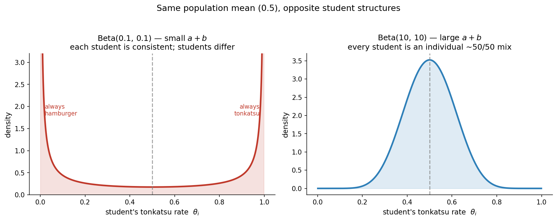
Same population mean, opposite stories about where the randomness lives. Let’s see it in samples: draw 5000 students from each population (each student gets a personal rate $\theta_i$ and brings 20 bentos) and measure the between-student spread.

 1
 2
 3
 4
 5
 6
 7
 8
 9
10
11
12
13
14
15
16
17
18
19
20
21
22
23
24
25

import jax
import jax.numpy as jnp
import jax.random as jr
from genjax import gen, beta, binomial

N_BENTOS = 20.0   # each student brings 20 bentos (a float so it shares a dtype
                  # with theta — GenJAX's binomial wants both the same type)

@gen
def student(a, b):
    theta = beta(a, b) @ "theta"          # this student's personal tonkatsu rate
    k = binomial(N_BENTOS, theta) @ "k"   # how many of their 20 bentos were tonkatsu
    return theta

def summarize(a, b, label, n_students=5000, seed=0):
    keys = jr.split(jr.key(seed), n_students)
    thetas = jax.vmap(lambda key: student.simulate(key, (a, b)).get_retval())(keys)
    print(label)
    print(f"  population mean rate        = {float(jnp.mean(thetas)):.2f}")
    print(f"  spread BETWEEN students (SD)= {float(jnp.std(thetas)):.2f}")
    print(f"  fraction near 0 or 1        = {float(jnp.mean((thetas < 0.1) | (thetas > 0.9))):.2f}")

summarize(0.1, 0.1, "Small a+b  -- Beta(0.1, 0.1):")
print()
summarize(10.0, 10.0, "Large a+b  -- Beta(10, 10):")

Output:

Small a+b  -- Beta(0.1, 0.1):
  population mean rate        = 0.50
  spread BETWEEN students (SD)= 0.46
  fraction near 0 or 1        = 0.81

Large a+b  -- Beta(10, 10):
  population mean rate        = 0.50
  spread BETWEEN students (SD)= 0.11
  fraction near 0 or 1        = 0.00

Both populations average $0.50$ tonkatsu — but in the small-$a+b$ world 81% of students are near-deterministic (always one or the other), while in the large-$a+b$ world none are: everybody is a genuine $50/50$ mix. The same point holds at any mean — make it $a:b = 7:3$ instead of $1:1$ and you get a population averaging $0.70$, either as “most students are reliably tonkatsu-or-hamburger people, leaning tonkatsu” (small $a+b$) or “every student personally brings tonkatsu about 70% of the time” (large $a+b$).

This is exactly what hierarchical Bayes infers. When we learn $(a, b)$ from data later in this chapter, we’re not just learning the average student — we’re learning the concentration, i.e. how much students differ, and that is precisely what decides how hard to shrink. A large inferred $a + b$ (students are alike) shrinks everyone hard toward the group; a small one (students differ) trusts each student’s own data more. Concentration is the knob that controls borrowing strength.

The reason the Beta is the prior for a rate is a happy algebraic accident called conjugacy — the prior and the posterior come out in the same family, so updating just shifts the parameters. You already met this in a different costume in Chapter 4: there, a Gaussian prior on a Gaussian mean gave a Gaussian posterior. Here, a Beta prior on a Bernoulli rate gives a Beta posterior — and the update is just counting:

$$\text{prior } \text{Beta}(a, b) ;+; \text{data } (k \text{ tonkatsu out of } n) ;\longrightarrow; \text{posterior } \text{Beta}(a + k,; b + n - k).$$

You add the observed tonkatsu to $a$ and the observed hamburgers to $b$. That’s the whole update. The posterior mean is therefore

$$\mathbb{E}[\theta \mid k, n] = \frac{a + k}{a + b + n},$$

which is exactly a blend of the prior soft-count and the real data — and, crucially, the blend tips toward the data as $n$ grows. Hold onto that formula; it is shrinkage, and the next section reads it off directly.