Markov Chain Monte Carlo: Designing a Chain to Hit a Target

Running Chapter 13 Backwards

In Chapter 13 we were handed a transition matrix $P$ — Chibany’s tonkatsu/hamburger habit — and asked a question: what is its stationary distribution $\pi$? We answered it two ways, by power iteration (just run the chain) and as the eigenvalue-1 eigenvector, and both landed on the same 70/30. The chain came first; the distribution $\pi$ fell out of it.

This chapter reverses the arrow.

Jamal: “Last week we started with a chain and found where it settles. But for inference I have the opposite problem. I know the distribution I want — it’s the posterior — I just can’t sample from it.”

Alyssa: “So you want to run the movie backwards. Instead of ‘here’s a chain, find its $\pi$,’ you want ‘here’s the $\pi$ I want, design me a chain that settles on it.’”

Jamal: “Can you even do that? Build a chain to order, so that its stationary distribution is whatever target I name?”

Alyssa: “You can. And the recipe is shorter than you’d think.”

That is Markov chain Monte Carlo (MCMC): given a target distribution $\pi$ — typically a Bayesian posterior we can evaluate but not sample — construct a Markov chain whose stationary distribution is exactly $\pi$. Run that chain, throw away the start, and the states it visits are samples from $\pi$. Recall the defining property of a stationary distribution from Chapter 13, $\pi P = \pi$: a single step leaves $\pi$ unchanged. MCMC is the art of building a $P$ that has your $\pi$ as its fixed point. Two recipes do it; we’ll meet both.

Metropolis–Hastings

The first recipe needs only the ability to evaluate the target (up to a constant) and to propose small moves. It is the Metropolis–Hastings (MH) algorithm, and it has just two moves per step.

Suppose the chain is currently at state $x$.

1. Propose a candidate next state $x'$ by drawing from a proposal distribution $Q(x' \mid x)$ — usually a small random nudge, $x' = x + \text{Gaussian noise}$.
2. Accept or reject. Compute the acceptance ratio $$A = \min\left(1, \frac{P(x')}{P(x)}\right),$$ and move to $x'$ with probability $A$; otherwise stay at $x$ (and record $x$ again).

graph LR
    A["current state x"] --> B["propose x' ~ Q(x'|x)"]
    B --> C{"u < min(1, P(x')/P(x)) ?"}
    C -->|accept| D["move to x'"]
    C -->|reject| E["stay at x"]
    D --> F["record the state"]
    E --> F
    F --> A
    classDef node fill:none,stroke:#9bbcff,stroke-width:2px,color:#fff
    class A,B,C,D,E,F node
    linkStyle default stroke:#9bbcff,stroke-width:2px,color:#fff

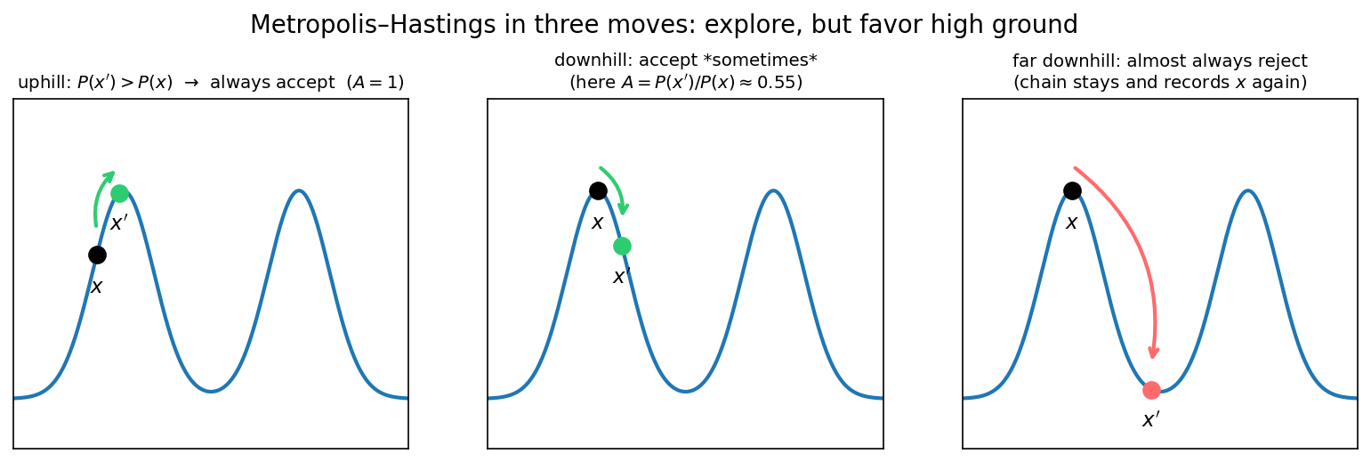
The intuition is exactly “explore, but favor high ground.” If $x'$ is more probable than $x$ ($P(x') > P(x)$), the ratio exceeds 1, $A = 1$, and you always move uphill. If $x'$ is less probable, you move only sometimes — with probability equal to the ratio of heights. So the chain wanders everywhere but spends most of its time where $P$ is large, which is precisely the behavior of a sample from $P$. Three snapshots of the rule in action:

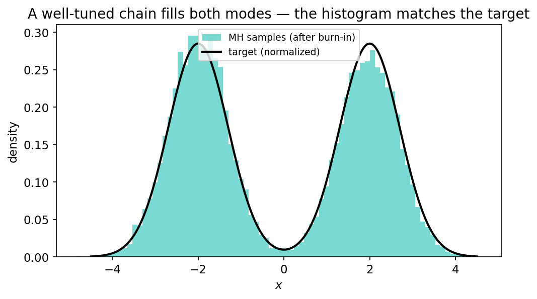
Here is MH on a deliberately hard target: a bimodal density with two well-separated peaks, at $-2$ and $+2$. A good proposal width lets the chain hop between both modes. We discard the first 2000 steps as burn-in — the early, pre-convergence portion before the chain has forgotten its arbitrary start.

 1
 2
 3
 4
 5
 6
 7
 8
 9
10
11
12
13
14
15
16
17
18
19
20
21
22
23
24
25

import jax
import jax.numpy as jnp
import jax.random as jr

def log_target(x):
    # unnormalized: a 50/50 mixture of two Gaussians, peaks at -2 and +2
    return jnp.log(0.5*jnp.exp(-0.5*((x+2)/0.7)**2) + 0.5*jnp.exp(-0.5*((x-2)/0.7)**2))

def mh(key, n_steps, step_sd, x0=0.0):
    def body(carry, k):
        x, n_acc = carry
        kp, ka = jr.split(k)
        x_prop = x + step_sd * jr.normal(kp)               # symmetric Gaussian proposal
        log_ratio = log_target(x_prop) - log_target(x)     # log P(x') - log P(x); normalizer cancels
        accept = jnp.log(jr.uniform(ka)) < log_ratio       # accept with probability min(1, ratio)
        x_new = jnp.where(accept, x_prop, x)
        return (x_new, n_acc + accept), x_new
    (_, n_acc), xs = jax.lax.scan(body, (x0, 0), jr.split(key, n_steps))
    return xs, float(n_acc) / n_steps

xs, acc = mh(jr.key(0), 20000, step_sd=1.5)
xs = xs[2000:]                                              # discard burn-in
print(f"acceptance rate: {acc:.2f}")
print(f"sample mean: {float(jnp.mean(xs)):.2f}  (target is symmetric about 0)")
print(f"fraction in the left mode: {float(jnp.mean(xs < 0)):.2f}  (~0.50 if well mixed)")

Output:

acceptance rate: 0.53
sample mean: -0.04  (target is symmetric about 0)
fraction in the left mode: 0.51  (~0.50 if well mixed)

The chain visits both peaks evenly — half its samples land on each side — and its mean sits at 0, the symmetric center. We never normalized the target; the acceptance ratio only ever used $\log P(x') - \log P(x)$. Pile the samples into a histogram and they trace out the target exactly:

Why the Normalizer Cancels

It is worth saying once, cleanly, why this is correct and not just plausible. A Metropolis–Hastings chain is built to satisfy a condition called detailed balance: the chain is equally likely to be found stepping from $x$ to $x'$ as from $x'$ to $x$, when $x$ is drawn from the target. A chain that satisfies detailed balance with respect to $P$ has $P$ as its stationary distribution — that is the theorem that makes the whole scheme work. (We’ll take it as a named fact rather than prove it.) The acceptance rule $A = \min(1, P(x')/P(x))$ is precisely the rule that forces detailed balance, and because it uses only a ratio, the normalizer drops out.

One simplification is worth naming. When the proposal is symmetric — $Q(x' \mid x) = Q(x \mid x')$, true for a Gaussian nudge — the proposal terms cancel too, and the acceptance ratio is just $P(x')/P(x)$. This special case is the original Metropolis algorithm; the general Hastings version carries an extra proposal-ratio correction for asymmetric proposals. Every chain in this chapter uses a symmetric proposal, so the clean $P(x')/P(x)$ form is all we need.

Gibbs Sampling

Metropolis–Hastings works for any target but throws some proposals away. The second recipe, Gibbs sampling, never rejects — at the cost of needing more from the model.

The idea: instead of proposing a joint move and accepting or rejecting it, update one coordinate at a time, drawing each from its exact conditional distribution given all the others. We need a piece of notation for “all the others”: write $x_{-i}$ to mean every coordinate except $i$ (the $-i$ is read “minus $i$”). The Gibbs update for coordinate $i$ is then

the conditional of coordinate $i$ given the current values of all the rest. Cycle through the coordinates, resampling each in turn, and the chain converges to the joint target.

Why does Gibbs always accept — no rejection step at all? Because sampling a coordinate from its true conditional automatically satisfies detailed balance with respect to the joint distribution. The conditional already “knows” the target along that axis, so there is nothing to correct: the acceptance probability works out to exactly 1. (Again a theorem; the intuition is that you proposed from exactly the right distribution, so you never need to throw the proposal away.) The price is that you must be able to sample each conditional — which is easy when the model is built from conjugate pieces, as we’ll see in Chapter 19.

Here is Gibbs on a correlated 2-D Gaussian (correlation $0.8$), whose two full conditionals are themselves simple Gaussians:

 1
 2
 3
 4
 5
 6
 7
 8
 9
10
11
12
13
14
15
16
17
18

import numpy as np

rho = 0.8
def gibbs(key, n_steps):
    def body(carry, k):
        x, y = carry
        kx, ky = jr.split(k)
        # full conditionals of a bivariate normal: x | y ~ N(rho*y, 1 - rho^2), and vice versa
        x = rho*y + jnp.sqrt(1 - rho**2) * jr.normal(kx)
        y = rho*x + jnp.sqrt(1 - rho**2) * jr.normal(ky)
        return (x, y), jnp.array([x, y])
    _, samples = jax.lax.scan(body, (0.0, 0.0), jr.split(key, n_steps))
    return samples

S = gibbs(jr.key(1), 20000)[1000:]                         # discard burn-in
cov = np.cov(np.array(S).T)
print(f"sample means: ({float(jnp.mean(S[:,0])):.2f}, {float(jnp.mean(S[:,1])):.2f})   (target 0, 0)")
print(f"sample correlation: {cov[0,1]/np.sqrt(cov[0,0]*cov[1,1]):.2f}        (target 0.8)")

Output:

sample means: (0.02, 0.02)   (target 0, 0)
sample correlation: 0.80        (target 0.8)

No proposal width to tune, no rejections — Gibbs recovers the means and the 0.8 correlation exactly. The moves are axis-aligned: each update slides along one coordinate while the other is held fixed, so the chain’s path is a staircase of little L-shaped steps climbing along the target’s ridge:

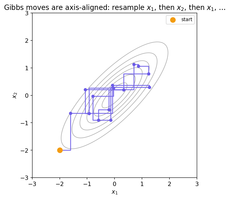
This is why a strongly correlated target can make Gibbs shuffle slowly along the diagonal — every move is parallel to an axis, so progress along the ridge takes many small steps.

MH vs Gibbs: Two Views

The two recipes trade off against each other cleanly:

In practice you often combine them — Gibbs for the coordinates whose conditionals are easy (conjugate), Metropolis for the ones that aren’t. That hybrid is exactly the sampler Chapter 19 builds for a real hierarchical model.

Mixing, Burn-In, and the Multimodal Trap

A subtlety hides in every MCMC run, and it is the difference between a correct sampler and a confidently wrong one. Two ideas pin it down.

The trace versus the histogram. When you run a chain for $N$ steps, you do not get $N$ independent samples. Each state is a small nudge from the last, so consecutive states are correlated. There are two ways to look at the output, and they answer different questions:

• The trace is the value plotted against iteration number — a time series. It shows you the chain’s journey: is it still drifting (not yet converged), or wandering steadily around a stable region (converged)?
• The posterior histogram batches all the post-burn-in states together, ignoring their order. That is your approximation to the target distribution.

You discard the early burn-in because those steps reflect the arbitrary starting point, not the target. And you remember that “10,000 steps” is worth fewer than 10,000 independent draws, because the steps are correlated.

Mixing. A chain has mixed when it has forgotten its start and is exploring the whole target — the same forgetting-the-start property we called ergodicity in Chapter 13. A well-mixed chain run twice from different starts gives the same answer. A badly mixed chain does not — and this is where multimodal targets bite.

Here is the trap. Take the same two-peaked target, but use a small proposal step, and run from the left mode and from the right mode separately:

1
2
3
4
5
6
7
8

xs_from_left,  _ = mh(jr.key(2), 20000, step_sd=0.3, x0=-2.0)   # start in the LEFT mode
xs_from_right, _ = mh(jr.key(3), 20000, step_sd=0.3, x0=+2.0)   # start in the RIGHT mode

frac_L = float(jnp.mean(xs_from_left[2000:]  < 0))
frac_R = float(jnp.mean(xs_from_right[2000:] < 0))
print(f"small step, started LEFT:  fraction in left mode = {frac_L:.2f}")
print(f"small step, started RIGHT: fraction in left mode = {frac_R:.2f}")
print("the two disagree -> the chain has NOT mixed (each is trapped near its start)")

Output:

small step, started LEFT:  fraction in left mode = 0.54
small step, started RIGHT: fraction in left mode = 0.19
the two disagree -> the chain has NOT mixed (each is trapped near its start)

The two runs flatly disagree — one thinks the target lives mostly on the left, the other mostly elsewhere — because the small step can never cross the low-probability valley between the peaks. Each chain is stuck in whichever mode it started in. The trace makes the diagnosis instant (drawn here at an even smaller step, $\sigma = 0.15$, where the trap is total):

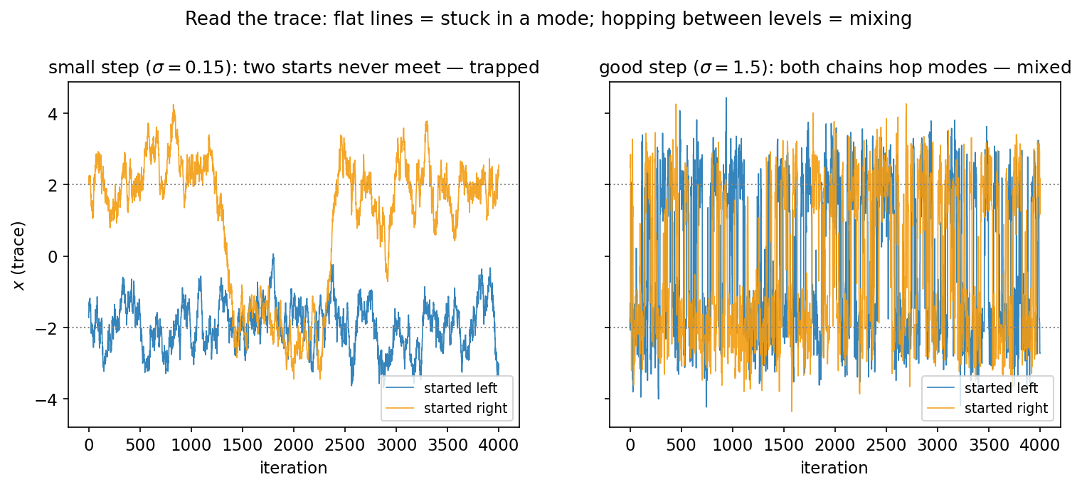
Crucially, the local acceptance rate looks perfectly healthy; the chain is happily accepting moves, just never the ones that would carry it across. Good local acceptance does not imply good global mixing. This is why multimodal posteriors are hard, and why diagnosing mixing — running multiple chains from different starts and checking they agree — matters.

Interactive: Watch a Chain Mix (or Get Trapped)

Everything in this section you can now see. The visualization below runs Metropolis–Hastings or Gibbs live on a multimodal 2-D Gaussian mixture (four well-separated blobs). The left panel shows the target density, the chain’s trail, and — for MH — the proposal circle with each proposal colored green (accepted) or red (rejected). The top-right panel is the trace (the x-coordinate against iteration: flat = stuck, hopping between levels = mixing); the bottom-right is the accumulated histogram against the true marginal. The readout in the corner gives the live acceptance ratio and a modes-visited counter — the honest “did it actually explore?” number.

(The same widget is used live in lecture; it is a single offline HTML file, so you can also open it full-screen to drive it with more room.)

In GenJAX

GenJAX has no black-box mh() in this version — and that is pedagogically perfect, because it means we assemble MH from the one primitive we need: a way to score a proposed state under the model. That primitive is assess. It takes a complete set of choices and returns the model’s log-probability of them — exactly the $\log P$ we feed into the acceptance ratio.

The model below is the small inference problem from the lecture: a prior $\mu \sim \mathcal{N}(0, 1)$, a likelihood $y \sim \mathcal{N}(\mu, 0.5)$, and one observation $y = 1.5$. Its posterior is known in closed form, $\mathcal{N}(1.2, 0.45^2)$, so we can check the sampler. We score each proposed $\mu$ (with $y$ fixed to the observation) using assess, form the ratio, and accept or reject.

 1
 2
 3
 4
 5
 6
 7
 8
 9
10
11
12
13
14
15
16
17
18
19
20
21
22
23
24
25
26
27
28

from genjax import gen, normal as gnormal, ChoiceMap

@gen
def model():
    mu = gnormal(0.0, 1.0) @ "mu"      # prior
    y  = gnormal(mu, 0.5) @ "y"        # likelihood
    return mu

def log_joint(mu, y_obs=1.5):
    logp, _ = model.assess(ChoiceMap.d({"mu": mu, "y": y_obs}), ())  # score the full trace
    return logp

def genjax_mh(key, n_steps, step_sd=0.5):
    def body(carry, k):
        mu, n_acc = carry
        kp, ka = jr.split(k)
        mu_prop = mu + step_sd * jr.normal(kp)
        log_ratio = log_joint(mu_prop) - log_joint(mu)   # y is fixed, so this is the posterior ratio
        accept = jnp.log(jr.uniform(ka)) < log_ratio
        mu_new = jnp.where(accept, mu_prop, mu)
        return (mu_new, n_acc + accept), mu_new
    (_, n_acc), mus = jax.lax.scan(body, (0.0, 0), jr.split(key, n_steps))
    return mus[2000:], float(n_acc) / n_steps

mus, acc = genjax_mh(jr.key(4), 20000)
print(f"acceptance rate: {acc:.2f}")
print(f"posterior mean of mu: {float(jnp.mean(mus)):.2f}   (closed form 1.20)")
print(f"posterior sd of mu:   {float(jnp.std(mus)):.2f}   (closed form 0.45)")

Output:

acceptance rate: 0.67
posterior mean of mu: 1.20   (closed form 1.20)
posterior sd of mu:   0.44   (closed form 0.45)

We built a correct posterior sampler out of one scoring call and a proposal — no normalizer, no closed-form posterior assumed. That assemble-it-yourself pattern is exactly what the next chapter scales up to a hierarchical model with many parameters.

Exercises

A companion notebook works through all of this interactively:

📓 Open in Colab: 18_markov_chain_monte_carlo.ipynb

Special thanks to JPPCA for their generous support of this tutorial series.