Monte Carlo: Estimating by Sampling

A Question You Can’t Sum

For three chapters now we have run Markov chains and watched where they settle. In Chapter 15 we ended on a promise: that running a chain to learn about a distribution is an idea with a name — Monte Carlo — and that the next part of the course turns it into a tool. This is that part.

Here is the kind of question that motivates it. Chibany eats two bentos a day, all semester, and their weights wander — some days a light onigiri set, some days a heavy katsu-and-rice. Jamal is curious.

Jamal: “What’s the average weight of one of your bentos this term?”

Chibany: “I’d have to add up every bento’s weight and divide by how many there were.”

Alyssa: “But you don’t have the list. And even if the weight were some smooth distribution, you’d have to do an integral — sum the weight times its probability over every possible weight. That’s a lot of adding.”

Alyssa has put her finger on the problem. The quantity Jamal wants is an expected value, and computing it exactly means summing (or integrating) over every possibility. For the bentos there are too many; for the Bayesian posteriors of Chapter 12, the integral has no closed form at all — which is exactly why that chapter’s importance sampling was, in its own words, “a blunt tool.”

There is a way out that needs no list and no integral. Sample, and average. That is the whole of Monte Carlo, and this chapter builds it up from a die roll to a tool sharp enough to estimate a probability you could never compute by hand.

The Monte Carlo Estimator

First, the thing we want. The expected value of a function $f$ of a random variable $X$ is its long-run average when $X$ is drawn from a distribution $P$. In the continuous case it is an integral,

which reads “add up $f(x)$, weighted by how likely each $x$ is.” (You met $\mathbb{E}$ for discrete sums back in Chapter 1; this is the same idea, with the sum become an integral.) We usually can’t do this integral. But we can estimate it. Draw $n$ independent samples $x_1, \dots, x_n$ from $P$ and average $f$ over them:

The hat on $\hat\mu_n$ means “estimated from a sample.” This is the Monte Carlo estimator, and the reason it works is a law you have already used informally every time you said “run it long enough”: the Law of Large Numbers guarantees that as $n$ grows, $\hat\mu_n$ converges to the true $\mathbb{E}_P[f(X)]$.

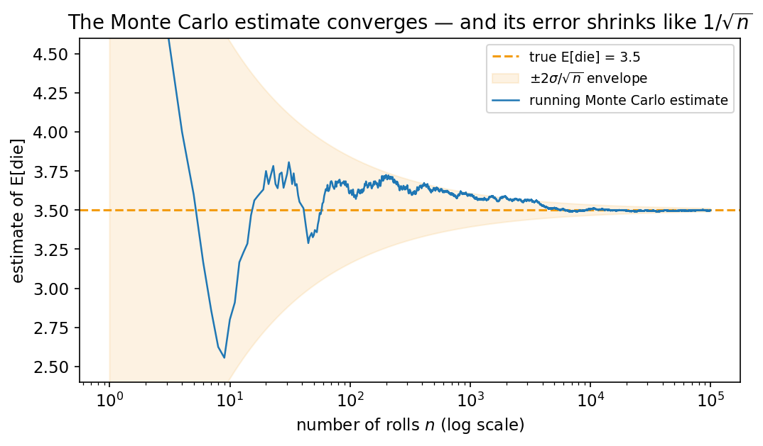
How fast? The error shrinks like $1/\sqrt{n}$: to halve your error you need four times as many samples. That sounds slow, but it has a remarkable property — the $1/\sqrt{n}$ rate doesn’t care how many dimensions $x$ lives in. A hand-summed integral gets exponentially harder as the dimension grows; Monte Carlo does not. That dimension-blindness is why it became the workhorse of modern statistics.

Watch it converge on the simplest possible expectation — the average roll of a fair die, whose true value is $\tfrac{1+2+3+4+5+6}{6} = 3.5$.

 1
 2
 3
 4
 5
 6
 7
 8
 9
10
11
12

import jax
import jax.numpy as jnp
import jax.random as jr

def die_estimate(key, n):
    rolls = jr.randint(key, (n,), 1, 7)        # n uniform draws from {1, ..., 6}
    return jnp.mean(rolls.astype(float))       # the Monte Carlo average

key = jr.key(0)
for n in [10, 100, 1000, 100000]:
    est = die_estimate(jr.fold_in(key, n), n)
    print(f"n = {n:6d}:  estimate of E[die] = {float(est):.3f}")

Output:

n =     10:  estimate of E[die] = 3.000
n =    100:  estimate of E[die] = 3.370
n =   1000:  estimate of E[die] = 3.484
n = 100000:  estimate of E[die] = 3.499

At $n=10$ the estimate is off by half a pip; by $n=100{,}000$ it is within a thousandth of $3.5$. We never wrote down “the average of a die is 3.5” — we discovered it by rolling. Here is the whole story in one picture — the running estimate wandering early, then funneling into 3.5 inside the shrinking $1/\sqrt{n}$ envelope:

Small Samples Swing Wide: the Hospital Problem

The $1/\sqrt{n}$ rate has a famous flip side, worth feeling before we move on. Here is a classic question (Kahneman & Tversky):

A large hospital (about 45 births a day) and a small hospital (about 15 births a day) each record, over a year, the days on which more than 60% of the babies born are boys. Which hospital records more such days?

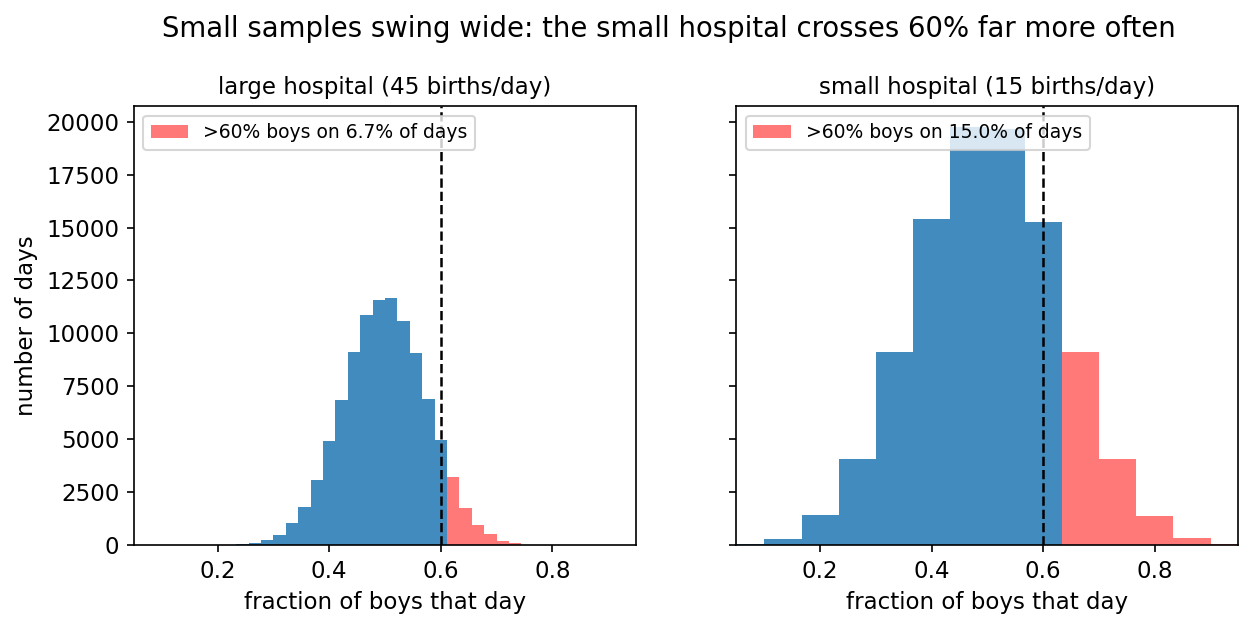
Most people say “about the same — boys are 50% everywhere.” But you now know better: $45$ births is a bigger sample than $15$, so the large hospital’s daily boy-fraction sits tight around 50%, while the small hospital’s swings wide — and crosses 60% far more often. Small samples vary more; that is the Law of Large Numbers, read in reverse. And notice the method we can use to check it: don’t compute anything — simulate a year and count. That move is Monte Carlo, applied to its own convergence.

1
2
3
4
5
6
7
8
9

def days_over_60(key, births_per_day, n_days=365):
    boys = jr.binomial(key, n=births_per_day * 1.0, p=0.5, shape=(n_days,))  # a year of days
    frac = boys / births_per_day
    return int(jnp.sum(frac > 0.6))                       # count the >60%-boys days

big   = days_over_60(jr.key(0), 45)
small = days_over_60(jr.key(1), 15)
print(f"large hospital (45 births/day): {big:3d} days over 60% boys")
print(f"small hospital (15 births/day): {small:3d} days over 60% boys")

Output:

large hospital (45 births/day):  27 days over 60% boys
small hospital (15 births/day):  55 days over 60% boys

The small hospital logs roughly twice as many lopsided days. Histogram a great many days and the mechanism is plain — the small hospital’s daily boy-fraction is simply a wider distribution, so far more of it pokes past the 60% line:

The same fact will return with teeth later in the chapter: an estimator built on effectively few samples swings wide in exactly this way.

π by Throwing Darts

The die was a warm-up: we knew the answer. Here is a Monte Carlo estimate of something you cannot get by counting — the number $\pi$ — using nothing but a stream of random points.

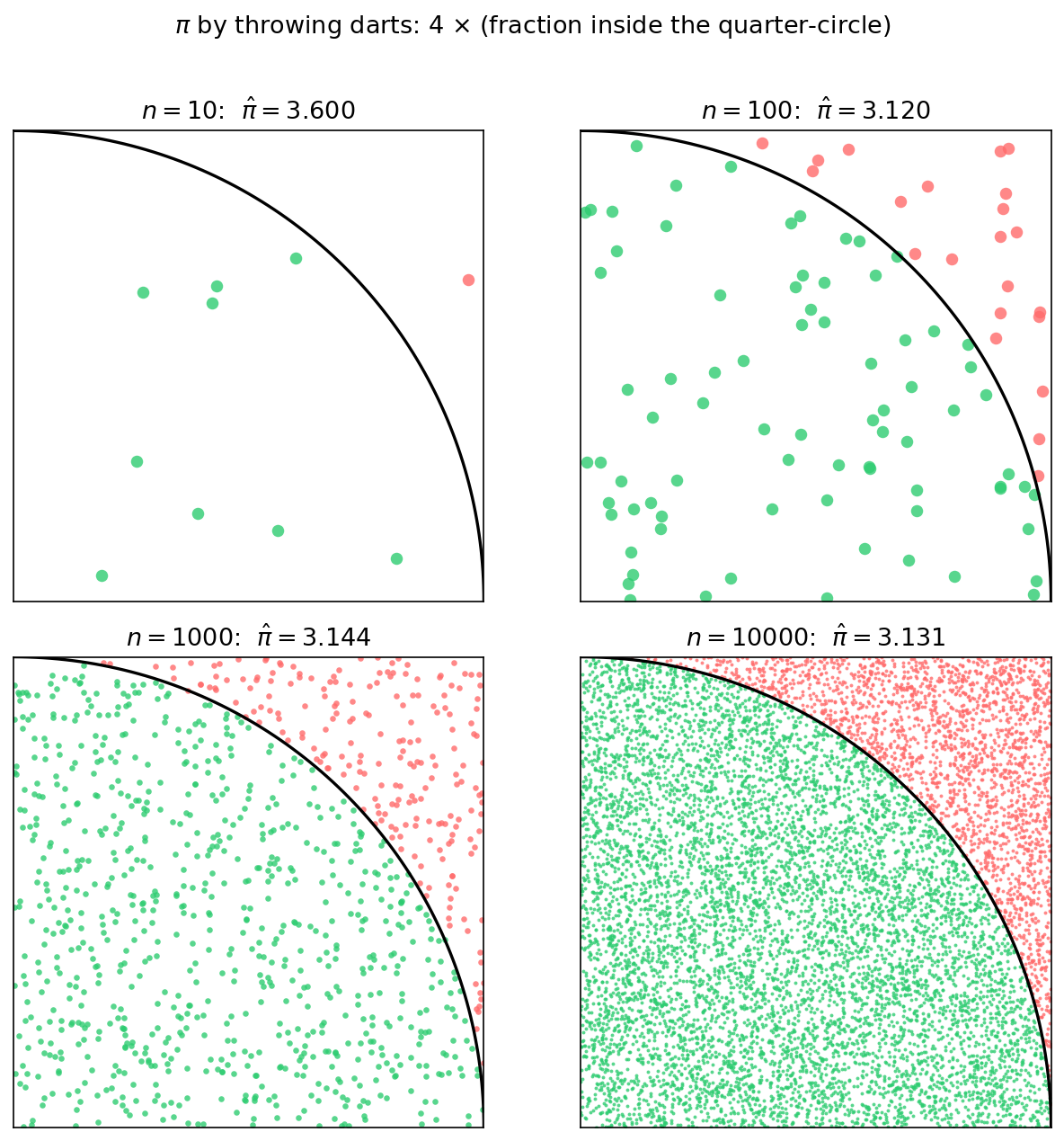
Picture the unit square $[0,1] \times [0,1]$ with a quarter-circle of radius 1 drawn inside it, centered at the corner. The square has area $1$; the quarter-circle has area $\tfrac{\pi}{4}$. So if you scatter darts uniformly over the square, the fraction that land inside the quarter-circle should be about $\tfrac{\pi}{4}$ — and four times that fraction estimates $\pi$.

To check whether a dart at $(x, y)$ is inside, we ask whether $x^2 + y^2 \le 1$. To turn that yes/no into a number we can average, we use the indicator function, written $\mathbb{1}[\cdot]$:

So $\mathbb{1}[x^2 + y^2 \le 1]$ is $1$ for darts inside the quarter-circle and $0$ for darts outside, and its average over many darts is the fraction inside. (Notice the move: a probability is just the expected value of an indicator. We’ll lean on that again and again.)

graph LR
    A["dart (x,y) ~ Uniform square"] --> B{"x² + y² ≤ 1 ?"}
    B -->|yes| C["1[inside] = 1"]
    B -->|no| D["1[inside] = 0"]
    C --> E["π̂ = 4 × average"]
    D --> E
    classDef node fill:none,stroke:#9bbcff,stroke-width:2px,color:#fff
    class A,B,C,D,E node
    linkStyle default stroke:#9bbcff,stroke-width:2px,color:#fff

1
2
3
4
5
6
7
8

def estimate_pi(key, n):
    xy = jr.uniform(key, (n, 2))                   # n darts in the unit square
    inside = (xy[:, 0]**2 + xy[:, 1]**2) <= 1.0    # indicator: inside the quarter-circle
    return 4.0 * jnp.mean(inside.astype(float)), int(jnp.sum(inside))

pi_hat, n_in = estimate_pi(jr.key(1), 100000)
print(f"darts inside the circle: {n_in} / 100000")
print(f"pi estimate = 4 x {n_in}/100000 = {float(pi_hat):.3f}")

Output:

darts inside the circle: 78345 / 100000
pi estimate = 4 x 78345/100000 = 3.134

A hundred thousand random darts pin $\pi$ to two decimal places. With the $1/\sqrt{n}$ rule, pinning the third decimal would take about a hundred times as many darts — slow, but utterly mechanical, and it never needed a single fact about circles beyond “inside means $x^2 + y^2 \le 1$.” Watch the picture sharpen as the darts accumulate:

And throw some darts yourself — watch the estimate’s path bounce hard at first, then calm down exactly as the $1/\sqrt{n}$ rule promises:

(Throw one dart at a time first — feel how jumpy the estimate is — then add ten thousand at once and watch it lock on.)

When You Can’t Sample P: Rejection and Inverse-CDF

Both examples so far sampled from something easy — a die, a uniform square. Real targets are rarely so cooperative. Two classic tricks turn “easy” samples into “hard” ones.

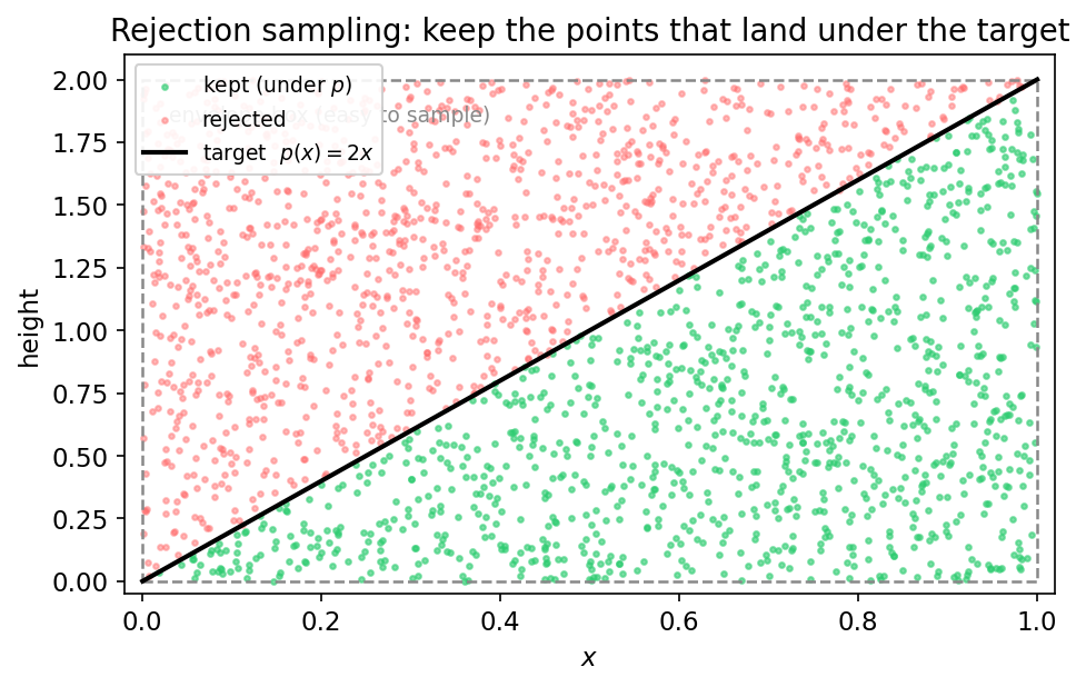
Rejection sampling. Suppose you can evaluate a target density $p(x)$ but not draw from it directly. Put a simple envelope over it — a box you can sample — throw points uniformly under the box, and keep only the points that fall under $p$. The survivors are exact samples from $p$; the rest are rejected. The catch is efficiency: if the box is much bigger than the area under $p$, you reject most of your work.

Here is a target shaped like a ramp, $p(x) \propto x$ on $[0,1]$ (a bento is more likely to be on the heavier side), sampled by rejection under a flat box of height 2.

 1
 2
 3
 4
 5
 6
 7
 8
 9
10

def rejection_sample(key, n_tries):
    kx, ky = jr.split(key)
    xs = jr.uniform(kx, (n_tries,))            # propose x ~ Uniform(0, 1)
    heights = jr.uniform(ky, (n_tries,)) * 2.0 # a height under the box (top = 2)
    keep = heights <= (2.0 * xs)               # accept if under p(x) = 2x
    return xs[keep], float(jnp.mean(keep))

samples, acc = rejection_sample(jr.key(2), 100000)
print(f"acceptance fraction: {acc:.3f}  (theory 0.5)")
print(f"kept {samples.shape[0]} samples; their mean = {float(jnp.mean(samples)):.3f}  (theory 2/3)")

Output:

acceptance fraction: 0.501  (theory 0.5)
kept 50077 samples; their mean = 0.667  (theory 2/3)

Half the proposals are thrown away — and the kept ones have mean $\tfrac{2}{3}$, exactly the mean of a ramp on $[0,1]$. Seen as a picture, the method is almost self-explanatory:

Inverse-CDF sampling. When you can write down the cumulative distribution $F(x) = P(X \le x)$ and invert it, there is no waste at all: draw $u \sim \text{Uniform}(0,1)$ and return $F^{-1}(u)$. Every uniform draw becomes one sample from the target. (You already did a one-step version of this in Chapter 13 — “draw $u$, compare to the row of the matrix” was inverse-CDF sampling of a two-outcome distribution.)

Rejection wastes samples when the envelope is loose. That waste is what the next idea fixes — not by throwing samples away, but by keeping all of them and adjusting their weight.

Importance Sampling: Sample the Wrong Distribution

Sometimes even an envelope is hard to find, or the region you care about is a tiny sliver that random sampling almost never visits. The fix is audacious: sample from a different, easier distribution on purpose, then correct for the lie.

To make this precise we need two distributions, and it is worth naming them clearly because the rest of the chapter — and the next two — lean on the distinction:

• the target $p(x)$ — the distribution we actually care about (often one we can evaluate but not easily sample), and
• the proposal $q(x)$ — an easy-to-sample stand-in that we draw from instead.

(You met a discrete version of this in Chapter 12, where the “proposal” was a finite grid of candidate priors. Here $q$ and $p$ are full continuous distributions that you get to choose.)

The trick is a single line of algebra. Multiply and divide by $q$:

So the expectation under $p$ equals an expectation under $q$, as long as we weight each sample by the importance weight

A good proposal $q$ looks like $p$ — broad where $p$ is broad, with weights that stay near 1. A bad proposal misses where $p$ lives, so a handful of samples get enormous weight and the rest get nearly zero. (Hold that thought; it becomes the chapter’s last idea.)

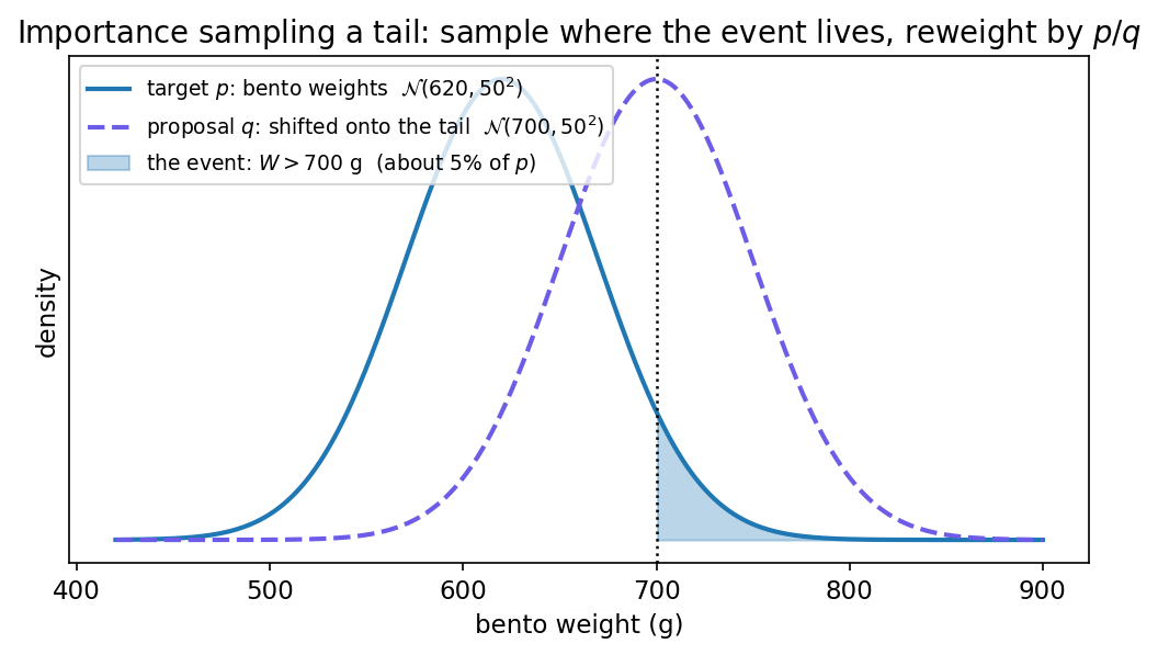
Here is the payoff example: estimating a tail probability that direct sampling would barely ever hit. Chibany’s bento weights follow $p = \mathcal{N}(620, 50^2)$ grams. What fraction of bentos top 700 g — a properly heavy lunch? Sampling from $p$ directly, only a few percent of draws clear 700, so the estimate is noisy. Instead we propose from $q = \mathcal{N}(700, 50^2)$, shifted onto the heavy tail, and reweight. The picture shows the move — the proposal parks itself right on top of the event:

 1
 2
 3
 4
 5
 6
 7
 8
 9
10
11
12
13
14
15

from jax.scipy.stats import norm

mu_p, sd_p = 620.0, 50.0      # target: where bento weights actually live
mu_q, sd_q = 700.0, 50.0      # proposal: shifted onto the heavy tail we care about

def is_tail(key, n):
    x = mu_q + sd_q * jr.normal(key, (n,))                    # sample from q
    w = norm.pdf(x, mu_p, sd_p) / norm.pdf(x, mu_q, sd_q)     # importance weight p/q
    f = (x > 700.0).astype(float)                            # indicator of "heavy bento"
    return float(jnp.mean(f * w))

est = is_tail(jr.key(3), 100000)
truth = float(1 - norm.cdf(700.0, mu_p, sd_p))
print(f"IS estimate of P(W > 700) = {est:.4f}")
print(f"true value                = {truth:.4f}")

Output:

IS estimate of P(W > 700) = 0.0542
true value                = 0.0548

By sampling where the action is and paying for it with weights, importance sampling estimates a tail probability cleanly. This is the move that powers the rest of the chapter — and it is exactly the lever the assignment asks you to pull on a different target of your own.

Self-Normalized IS and Unnormalized p

There is a subtle, enormously useful variant. In Bayesian inference the target is a posterior, $p(x) = \tfrac{1}{Z}\tilde p(x)$, and the normalizing constant $Z = p(\text{data})$ is precisely the integral we cannot compute. Watch what happens if we only ever take ratios of weights:

The unknown $Z$ appears in every weight identically, so it cancels between numerator and denominator. This is the self-normalized estimator, and it means you can do importance sampling with an unnormalized target — exactly the situation every posterior puts you in. (This cancellation is the same one that will make MCMC work in Chapter 18.)

Here it is on a coin: a $\text{Beta}(2,2)$ prior on the head-probability $\theta$, one observed head, recovering the posterior mean.

1
2
3
4
5
6
7
8

def snis_coin(key, n):
    theta = jr.beta(key, 2.0, 2.0, (n,))   # sample theta from the PRIOR (our proposal q)
    w = theta                              # likelihood of one head is theta, so w is proportional to it
    return float(jnp.sum(theta * w) / jnp.sum(w))   # self-normalized: the constant cancels

post_mean = snis_coin(jr.key(4), 200000)
print(f"self-normalized IS posterior mean of theta = {post_mean:.3f}")
print(f"closed form (Beta(3,2) mean = 3/5)         = {3/5:.3f}")

Output:

self-normalized IS posterior mean of theta = 0.601
closed form (Beta(3,2) mean = 3/5)         = 0.600

Likelihood Weighting

That coin example hid a beautiful special case. We chose the proposal $q$ to be the prior. When $q = p(\text{hypothesis})$, the importance weight collapses to

the likelihood. So “sample from the prior, weight by the likelihood” is importance sampling with the prior as proposal — and it is exactly what Chapter 12 did when it called importance sampling “a blunt tool.” Blunt, because the prior is often a poor proposal: it scatters samples broadly, the likelihood concentrates the weight onto a few, and the estimate gets noisy. How noisy? That has a diagnostic — but first, a cognitive aside that will recur all term.

Exemplar Models Are Importance Samplers

One of the most successful models of human categorization answers questions by a similarity-weighted vote over stored examples. In an exemplar model (Nosofsky, 1986), you don’t carry around an abstract rule for “tonkatsu bento” — you carry around the bentos you remember, and when a new one arrives you ask each memory how similar it is:

where $s(x, x_i)$ is the similarity between the query $x$ and stored example $x_i$, and $f(x_i)$ is the label stored with example $i$ (say, 1 for tonkatsu, 0 for not).

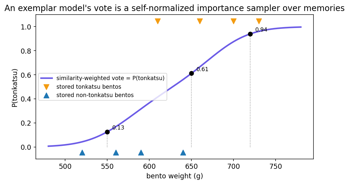
Look hard at that formula. It is exactly the self-normalized importance-sampling estimator from a few sections ago, $\sum_i w_i f(x_i) / \sum_i w_i$ — with the stored exemplars playing the role of the samples and the similarity $s$ playing the role of the weight $w$. A mind that classifies by similarity-weighted voting over memories is, mechanically, running an importance sampler over its own experience. Here it is deciding whether a new bento is tonkatsu from its weight:

 1
 2
 3
 4
 5
 6
 7
 8
 9
10

# Chibany's memory of past bentos: weight (g) and whether it was tonkatsu (1) or not (0).
weights = jnp.array([520., 560., 590., 610., 640., 660., 700., 730.])
is_tonk = jnp.array([0.,   0.,   0.,   1.,   0.,   1.,   1.,   1.])

def exemplar_vote(x, width=40.0):
    s = jnp.exp(-0.5 * ((x - weights) / width) ** 2)   # similarity to each stored example
    return float(jnp.sum(s * is_tonk) / jnp.sum(s))   # similarity-weighted vote

for query in [550.0, 650.0, 720.0]:
    print(f"a {query:.0f} g bento: P(tonkatsu) by exemplar vote = {exemplar_vote(query):.2f}")

Output:

a 550 g bento: P(tonkatsu) by exemplar vote = 0.13
a 650 g bento: P(tonkatsu) by exemplar vote = 0.61
a 720 g bento: P(tonkatsu) by exemplar vote = 0.94

Light bentos vote “not tonkatsu,” heavy ones vote “tonkatsu,” and the middle hedges — a graded generalization curve, produced by nothing but weighted memories:

This bridge — a classic process model of cognition is a Monte Carlo estimator in disguise — is the first of several in these chapters; Chapter 17 and Chapter 19 push it much further.

Effective Sample Size

When a few weights dominate, your thousand weighted samples are not worth a thousand even ones — most carry almost no weight. The effective sample size measures how many samples are really pulling their weight. With normalized weights $w_t$ (so $\sum_t w_t = 1$),

Read the two extremes:

• Perfectly even weights ($w_t = 1/T$ for all $t$): $\sum_t w_t^2 = T \cdot (1/T)^2 = 1/T$, so $N_{\text{eff}} = T$. Every sample counts fully.
• One weight dominates ($w_1 \approx 1$, the rest $\approx 0$): $\sum_t w_t^2 \approx 1$, so $N_{\text{eff}} \approx 1$. A thousand samples worth one.

So $N_{\text{eff}}$ is a diagnostic of how evenly the weights are spread — equivalently, of how well your proposal $q$ matches the target $p$. A well-matched $q$ gives near-even weights and $N_{\text{eff}}$ close to $T$; a mismatched $q$ collapses the weight onto a few samples and $N_{\text{eff}}$ crashes. Watch it on Chibany’s bento target with two proposals — one shaped like $p$, one badly off in the tail and too narrow.

 1
 2
 3
 4
 5
 6
 7
 8
 9
10

def ess_of(key, mu_q, sd_q, n=100000):
    x = mu_q + sd_q * jr.normal(key, (n,))
    logw = norm.logpdf(x, mu_p, sd_p) - norm.logpdf(x, mu_q, sd_q)  # log importance weight
    w = jnp.exp(logw - jnp.max(logw)); w = w / jnp.sum(w)           # normalize the weights
    return float(1.0 / jnp.sum(w**2))                              # effective sample size

ess_good = ess_of(jr.key(5), 630.0, 55.0)   # q close to p
ess_poor = ess_of(jr.key(6), 760.0, 30.0)   # q far out in the tail, too narrow
print(f"well-matched q ~ N(630,55):   ESS = {ess_good:8.0f}  out of 100000")
print(f"poorly-matched q ~ N(760,30): ESS = {ess_poor:8.0f}  out of 100000")

Output:

well-matched q ~ N(630,55):   ESS =    95719  out of 100000
poorly-matched q ~ N(760,30): ESS =       22  out of 100000

A well-matched proposal keeps almost all of its 100,000 samples; a badly-matched one is left with the worth of 22. The contrast is easiest to see side by side — when the proposal misses the target, the weight histogram collapses into a spike of near-zeros dominated by a handful of giants:

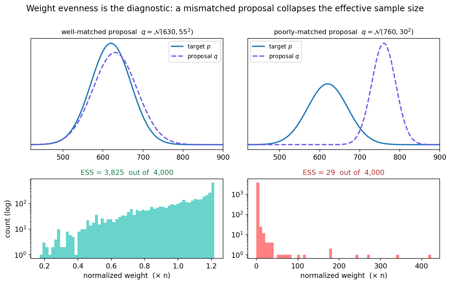
That is what $N_{\text{eff}}$ is for: a quick read on whether your proposal covers your target. Now build the feel for it with your own hands — drag the proposal around and watch the weights and the ESS respond:

(Try three positions: the proposal right on the target; far off in a tail; and parked on the shaded $W > 700$ event. Watch both readouts each time.)

In GenJAX

Everything above we hand-rolled. GenJAX gives importance sampling as a built-in: a model’s importance method draws from a proposal and returns the sample together with its log-weight. You have seen simulate and generate in earlier chapters; importance is the new primitive here.

model.importance(key, constraint, args) runs the model forced to agree with the observations in constraint, samples the unobserved choices from the model’s prior, and returns (trace, log_weight) — the log of the importance weight you would otherwise compute by hand. Constrain the observed head to True, draw $\theta$ from the prior, self-normalize the log-weights, and the posterior mean falls out.

 1
 2
 3
 4
 5
 6
 7
 8
 9
10
11
12
13
14
15
16
17
18

from genjax import gen, beta as gbeta, flip, ChoiceMap

@gen
def coin_model():
    theta = gbeta(2.0, 2.0) @ "theta"     # prior over the head-probability
    head  = flip(theta) @ "head"          # one coin flip
    return theta

def genjax_snis(key, n):
    keys = jr.split(key, n)
    def one(k):
        tr, lw = coin_model.importance(k, ChoiceMap.d({"head": True}), ())  # observe a head
        return tr.get_choices()["theta"], lw
    thetas, lws = jax.vmap(one)(keys)
    w = jnp.exp(lws - jnp.max(lws)); w = w / jnp.sum(w)   # self-normalize the weights
    return float(jnp.sum(w * thetas))

print(f"GenJAX self-normalized IS posterior mean = {genjax_snis(jr.key(7), 200000):.3f}  (closed form 0.600)")

Output:

GenJAX self-normalized IS posterior mean = 0.600  (closed form 0.600)

Same answer as our hand-rolled version, with the weight bookkeeping handled for you. (For a custom proposal that isn’t the prior, GenJAX gives model.assess(choices, args) to score any chosen sample — we’ll use that scoring primitive to build MCMC in Chapter 18.)

Exercises

A companion notebook works through all of this interactively:

📓 Open in Colab: 16_monte_carlo.ipynb

References

• Nosofsky, R. M. (1986). Attention, similarity, and the identification–categorization relationship. Journal of Experimental Psychology: General, 115(1), 39–61. https://doi.org/10.1037/0096-3445.115.1.39
• Tversky, A., & Kahneman, D. (1974). Judgment under uncertainty: Heuristics and biases. Science, 185(4157), 1124–1131. https://doi.org/10.1126/science.185.4157.1124

Special thanks to JPPCA for their generous support of this tutorial series.