Particle Filtering: Yesterday's Posterior Is Today's Prior
Why this chapter (and a note on the assignment)
Chapter 16 estimated a fixed quantity — the average bento, a tail probability — from a batch of samples. But data often arrive one at a time, and the thing you’re estimating moves. This chapter adapts importance sampling to that streaming case. It is not needed for the Monte Carlo assignment, but it is the natural bridge between the Monte Carlo of Chapter 16 and the Markov chain Monte Carlo of Chapter 18 — and it is where sampling becomes a model of how a mind might track a changing world in real time.
Following Chibany Down the Corridor
Chibany is walking down a long corridor to the lab, and Jamal — sitting at his desk — is trying to figure out where they are from a noisy sensor over the door that pings a rough distance reading every few seconds.
Jamal: “The pings are all over the place. One says 1.3 meters, the next 1.8, then a jump to 3.4. I can’t trust any single one.”
Alyssa: “You don’t have to. You know two things the sensor doesn’t: Chibany keeps walking forward at a steady pace, and each ping is the true position plus a bit of noise. Use both.”
Jamal: “So at every ping I update my guess — and my guess from a moment ago becomes my starting point for the next?”
Alyssa: “Exactly. Yesterday’s answer is today’s question.”
Alyssa has described sequential inference, and the tool for it is a swarm of weighted Monte Carlo samples that crawls along behind the moving target. Let us set up the pieces, then build it.
Data Arriving One at a Time
Two ingredients turn “a noisy sensor” into a model. They are the standard furniture of a state-space model — a hidden thing that evolves, observed only through noise.
- The hidden state $x_t$ — what we actually want to know (Chibany’s true position at tick $t$). We never see it directly.
- The motion model $p(x_t \mid x_{t-1})$ — how the state evolves. Here, Chibany steps forward about 1 meter per tick, with a little wobble: $x_t = x_{t-1} + 1 + \text{noise}$.
- The observation model $p(z_t \mid x_t)$ — how a noisy reading $z_t$ relates to the true state. Here, the ping is the true position plus sensor noise: $z_t \sim \mathcal{N}(x_t, \sigma_{\text{obs}}^2)$.
Both models are choices — assumptions we make about the world. Given them, the goal is the posterior over the current state given all the pings so far, $p(x_t \mid z_1, \dots, z_t)$. The key that makes this tractable in a stream is a recursion:
$$p(x_t \mid z_1, \dots, z_t) \propto p(z_t \mid x_t) \underbrace{p(x_t \mid z_1, \dots, z_{t-1})}_{\text{predicted from yesterday}}.$$Read it right to left. Take yesterday’s posterior, push it forward through the motion model to predict where Chibany is now — that prediction is today’s prior. Then weight by how well each possibility explains today’s ping, the likelihood $p(z_t \mid x_t)$. The product (up to a constant) is today’s posterior. Yesterday’s posterior is today’s prior — that single sentence is the whole algorithm.
Sequential Importance Sampling
We can’t write that posterior down in closed form, but Chapter 16 already taught us what to do when we can’t: represent the distribution by a cloud of samples and reweight. Here the cloud is a set of particles — $M$ candidate values of the hidden state, each a little guess about where Chibany is — and we apply importance sampling once per tick. That repeated, streaming importance sampling is called sequential importance sampling (SIS), and dressed up with one extra step it becomes the particle filter.
graph LR
    A["M particles<br/>(guesses of x_t)"] --> B["WEIGHT<br/>w ∝ p(z_t | x_i)"]
    B --> C["RESAMPLE<br/>keep heavy, drop light"]
    C --> D["PROPAGATE<br/>x ~ p(x_t+1 | x_t)"]
    D --> A
    classDef node fill:none,stroke:#9bbcff,stroke-width:2px,color:#fff
    class A,B,C,D node
    linkStyle default stroke:#9bbcff,stroke-width:2px,color:#fff
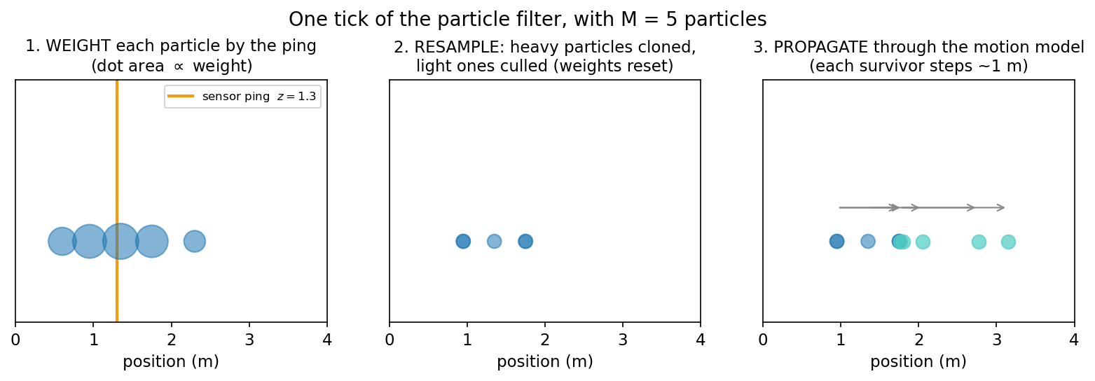
The loop has three moves, and each maps onto an idea you already have:
- Weight. Score every particle by the likelihood of the new ping: $w_i \propto p(z_t \mid x_i)$. A particle near the true position explains the ping well and earns a big weight; a particle far off earns almost nothing. (This is exactly the importance weight of Chapter 16, applied to one new observation.)
- Resample. Here is the new move. Resampling means drawing $M$ new particles from the old ones, with probability proportional to their weights: a particle with weight $0.4$ is, on average, copied twice; a particle with weight $0.001$ almost certainly vanishes. Concretely, it is a single $\text{Categorical}(\text{normalized weights})$ draw of $M$ indices. After resampling, all particles have equal weight again — the heavy ones have simply been cloned and the light ones culled, so the swarm concentrates where the action is.
- Propagate. Push each surviving particle forward through the motion model, $x \sim p(x_{t+1} \mid x_t)$. Now the cloud is a fresh set of guesses for the next tick — yesterday’s posterior, become today’s prior. Loop.
Here is one full tick of the loop, drawn with just five particles so every move is visible:
Better still, drive the loop yourself. The widget below runs the exact corridor episode from the worked example coming up — same pings, same models — one phase per click, narrating which move it just made:
(Step through a full episode at M = 200. Then switch to M = 20 and run it again a few times — watch the estimate get jumpier with fewer particles. That wobble is the “limited memory” theme of the last section, made visible.)
Worked Example: Tracking on a Line
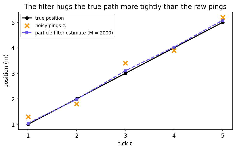
Let us actually follow Chibany. The true positions are $1, 2, 3, 4, 5$ (one meter per tick); the sensor reports the noisy pings $1.3, 1.8, 3.4, 3.9, 5.2$. We run $M = 2000$ particles, init them near the start, and step the weight–resample–propagate loop once per ping, recording the weighted-mean estimate each time.
| |
Output:
true positions : [1.0, 2.0, 3.0, 4.0, 5.0]
noisy pings    : [1.3, 1.8, 3.4, 3.9, 5.2]
filter estimate: [1.04, 1.98, 3.1, 4.03, 5.08]
The filter’s estimate hugs the true line $[1, 2, 3, 4, 5]$ far more tightly than the raw pings do — it smooths the noise by combining each ping with the steady-march prior. That is the payoff of using both models the sensor doesn’t know about:
Resampling and Degeneracy
Why is resampling — step 2 — not optional? Skip it, and you have plain sequential importance sampling: weight, then propagate, never culling. The trouble is that weights multiply over time. After many ticks, one lucky particle accumulates almost all the weight and every other particle is carrying essentially zero — the swarm has collapsed to a single point pretending to be a distribution. This is weight degeneracy, and the effective sample size from Chapter 16 measures it exactly. Watch it crash as the track gets longer, without resampling:
| |
Output:
T =  5 steps, no resampling:  ESS =   957.5  / 2000
T = 10 steps, no resampling:  ESS =   421.4  / 2000
T = 20 steps, no resampling:  ESS =    61.2  / 2000
By 20 steps, 2000 particles are worth about 61 — the rest are dead weight. Extend the track further and the collapse just keeps going:
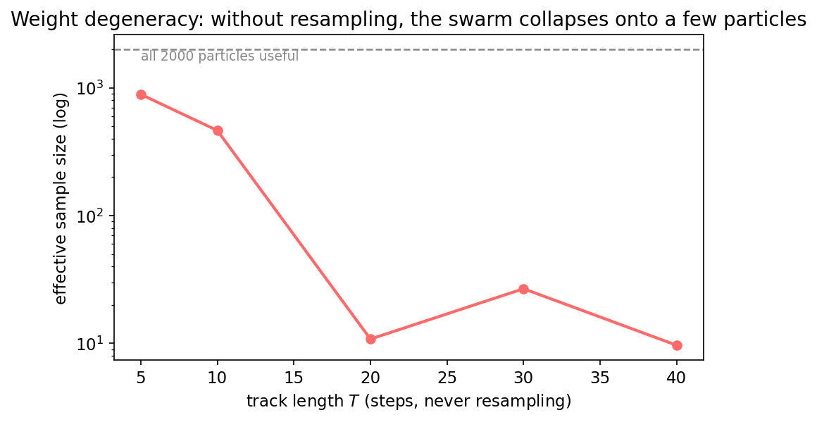
Resampling is the cure: by culling the no-hope particles and cloning the promising ones at every tick, it keeps the whole swarm useful, so the filter can run indefinitely without collapsing.
Particles as a Process Model
Here is where this stops being an algorithm and starts being psychology. A particle filter does not hold the full posterior — it holds a finite handful of guesses and updates them under a strict left-to-right pass over the data. That sounds like a limitation. It is also a remarkably good description of how people track a changing world, and the match is the point.
Think about what a small particle filter predicts about a fallible reasoner:
- Limited memory. With only $M$ particles, the swarm can represent only so much uncertainty at once — like a person juggling a few live hypotheses, not a probability distribution over all of them. $M$ becomes a knob you can fit to data: how many guesses is a person effectively running?
- Order effects. Because early data can kill off particles that later data would have vindicated, a particle filter is sensitive to the order in which evidence arrives — and so are people.
- Run-to-run variability. Resampling is stochastic, so two runs on the same data can land differently — mirroring the genuine variability in human judgments.
This is the rational process model idea: the same Bayesian computation, run under a realistic resource budget, predicts not just the right answer but the characteristic ways people deviate from it. Particle filters in particular have been used to model human category learning, associative learning, and online sentence processing (Sanborn, Griffiths & Navarro 2010; Austerweil & Griffiths 2013, among others) — sampling not as a numerical convenience, but as a hypothesis about the mind.
In GenJAX
The hand-rolled filter spelled out all three moves. GenJAX lets us write the propagate step as a tiny generative model — the motion model is a @gen function — and reuse the weight-and-resample logic around it. The structure is identical; only the propagate line changes.
| |
Output:
genjax filter estimate: [1.04, 1.98, 3.1, 4.03, 5.08]Same track, same answer. (GenJAX’s smc module packages this whole loop — weighting, resampling, propagating — into a reusable sequential-Monte-Carlo routine; the hand-rolled version here is exactly what it automates.)
What you can do now
You can set up a state-space model — a hidden state with a motion model and an observation model — and recognize the recursion that makes streaming inference work: yesterday’s posterior is today’s prior. You can run a particle filter: represent the posterior with a swarm of weighted particles and loop weight → resample → propagate, where resampling is a Categorical draw that clones heavy particles and culls light ones to defeat weight degeneracy. And you can see why a small particle filter is a candidate process model of human inference — limited memory, order effects, and variability falling out of the resource budget.
Next, Chapter 18 keeps the target fixed but makes the samples themselves into a Markov chain — running Chapter 13 backwards to design a chain whose stationary distribution is whatever posterior we want.
Glossary: particle filter, resampling, importance sampling, effective sample size. 🔧 log-sum-exp trick, self-normalized importance weights.
Exercises
Try it yourself
- Shrink the swarm. Re-run the tracking filter with $M = 20$ particles instead of 2000. Does it still track the line? Run it a few times with different keys — how much does the estimate wobble run to run? Relate what you see to “limited memory” and “run-to-run variability.”
- Turn off resampling. Modify
filter_stepto skip the resample line (propagate the weighted particles directly, carrying weights forward). On the 5-step track it may look fine; extend to a 30-step track and compare the estimate’s accuracy to the resampling version. What goes wrong, and why? - A noisier sensor. Double
OBS_SDto 1.4 (much noisier pings). Predict first: should the filter’s estimate get closer to the raw pings or stay closer to the steady-march prior? Run it and check.
A companion notebook works through all of this interactively:
📓 Open in Colab: 17_particle_filtering.ipynb
References
- Austerweil, J. L., & Griffiths, T. L. (2013). A nonparametric Bayesian framework for constructing flexible feature representations. Psychological Review, 120(4), 817–851. https://doi.org/10.1037/a0034194
- Sanborn, A. N., Griffiths, T. L., & Navarro, D. J. (2010). Rational approximations to rational models: Alternative algorithms for category learning. Psychological Review, 117(4), 1144–1167. https://doi.org/10.1037/a0020511
Special thanks to JPPCA for their generous support of this tutorial series.