Sampling the Mind: People and the Kemp Hierarchy
A note on this chapter and the assignment
This chapter teaches the full method — a working Gibbs-plus-Metropolis sampler for a hierarchical model — but on a different application (Chibany rating bento shops) and with different data and a different derivation than the Monte Carlo assignment. That is deliberate: you should finish here able to build such a sampler, then meet a fresh version of the problem on the assignment, so you are exercising the skill rather than copying an answer. Where the assignment goes somewhere this chapter does not, we’ll say so plainly.
When a Person Is the Accept Step
Chapter 18 built Metropolis–Hastings out of one move: propose a change, then accept it with a probability that compares the new state to the old. Here is a strange and beautiful question.
Alyssa: “Show someone two slightly different cartoon animals and ask ‘which looks more like a cat?’ They pick one. Then you tweak it, ask again, they pick again. What are they doing, step by step?”
Jamal: “Proposing a change, and accepting it if it looks more cat-like… that’s the Metropolis accept step. The person is the accept step.”
Alyssa: “And if the person accepts in proportion to how well each option fits their idea of ‘cat’ — then the sequence of choices is a Markov chain. What’s its stationary distribution?”
If a learner accepts proposals in proportion to their own posterior $P(h \mid \text{data})$, then by the logic of Chapter 18 the chain over hypotheses $h$ converges to that posterior as its stationary distribution. And here is the twist that makes it a measurement tool: run the procedure with no data to fit, just “which looks more like a cat,” and the posterior is the person’s prior — their mental concept of “cat.” The chain converges to the shape of an idea inside someone’s head. You can read out a person’s prior by running them as MCMC.
This is Markov chain Monte Carlo with People (Sanborn & Griffiths, 2007). Run on cartoon animals — stick-figure giraffes, horses, cats, dogs whose proportions are a handful of numbers — it recovers each category’s mental prototype as the stationary distribution of people’s choices, and the four categories come out cleanly separated in the recovered space. The sampler of the last chapter, pointed at a person, becomes an instrument for cognition.
The rest of this chapter points the same machinery at a different target: not a person’s prior, but the posterior of a hierarchical model — the one Chapter 12 set up and could only approximate bluntly. Now we can sample it sharply.
A Sampler for the Bento-Shop Hierarchy
Chibany has been rating bento shops. For each shop $i$, they record $k_i$ good tonkatsu ratings out of $n_i$ visits. Each shop has its own true tonkatsu-quality rate $\theta_i$ — but the shops are not unrelated: they are all in the same city, and Chibany suspects there is a population pattern — a typical quality, and a typical spread around it — that the shops are drawn from.
This is exactly the two-level Beta-Binomial hierarchy of Chapter 12:
$$\theta_i \sim \text{Beta}(a, b), \qquad k_i \sim \text{Binomial}(n_i, \theta_i),$$with the population prior $(a, b)$ itself learned from all the shops together (Chapter 12’s overhypothesis idea — the prior is acquired, not assumed). Chapter 12 estimated this with importance sampling and called it “a blunt tool,” noisy because the prior is a poor proposal. We will now sample the posterior with MCMC instead. Here is the whole model as a picture:
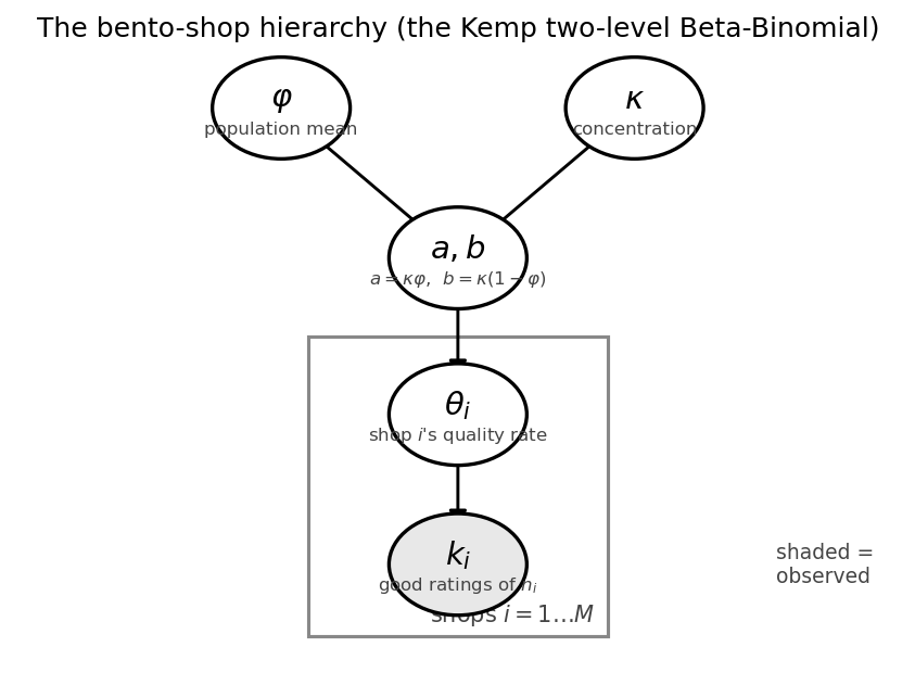
The reparametrization. The natural Beta parameters $(a, b)$ are awkward for a sampler: they can sit at wildly different scales (maybe $a = 2$, $b = 30$), and they tangle two distinct ideas together. So we switch to a pair that separates those ideas:
- $\varphi = \dfrac{a}{a+b} \in (0, 1)$ — the mean quality (where the population is centered), and
- $\kappa = a + b > 0$ — the concentration (how tightly shops cluster around that mean: large $\kappa$ = all shops alike, small $\kappa$ = shops all over the map).
We sample one more level down, in $\ell = \log \kappa$, so that the concentration stays positive automatically and a symmetric random-walk step behaves sensibly. Three numbers — $(\varphi, \ell)$ plus the per-shop $\theta_i$ — same model, but now each knob means one clean thing.
Get a feel for the two knobs before we sample them. The explorer below draws the population prior $\text{Beta}(\kappa\varphi, \kappa(1-\varphi))$ as you drag $\varphi$ and $\kappa$ — watch how the mean slides the bump while the concentration changes its whole character, from “every shop is extreme” (U-shaped, $\kappa < 1$) to “all shops identical” (a spike):
(Slide $\kappa$ from one extreme to the other while holding $\varphi$ at 0.6 — that single knob is what the Metropolis step will be learning from the shops.)
The plan is a hybrid sampler, exactly the MH-and-Gibbs combination Chapter 18 pointed at: Gibbs for the part that’s conjugate and easy, Metropolis for the part that isn’t.
graph LR
    A["Gibbs: redraw each θ_i<br/>from its conjugate Beta"] --> B["Metropolis: propose (φ', ℓ')<br/>accept by marginal-likelihood ratio"]
    B --> A
    classDef node fill:none,stroke:#9bbcff,stroke-width:2px,color:#fff
    class A,B node
    linkStyle default stroke:#9bbcff,stroke-width:2px,color:#fff
Step 1 — Gibbs the θᵢ (Conjugate)
The per-shop rates are the easy part. Hold the population $(a, b)$ fixed; then each $\theta_i$ depends only on its own shop’s data, and the Beta-Binomial conjugacy from Chapter 12 gives its full conditional in closed form:
$$\theta_i \mid a, b, k_i, n_i \sim \text{Beta}(a + k_i,\ b + n_i - k_i).$$This is a direct draw from the exact conditional — a Gibbs step. As in Chapter 18, there is no accept/reject: sampling from the true conditional always accepts.
| |
Output:
one Gibbs draw of theta_i: [0.9, 0.47, 0.54, 0.33, 0.68, 0.17, 0.52, 0.88, 0.43, 0.62, 0.27, 0.9]Each shop’s rate is pulled toward its own data (shop 1 with 9/10 lands high, shop 11 with 1/10 lands low), but also shrunk toward the population — exactly the partial pooling of Chapter 12, now happening one Gibbs draw at a time.
Integrating Out θᵢ: the Beta-Binomial Marginal
The population $(\varphi, \kappa)$ is the hard part, because its conditional is not a tidy named distribution. But there is a clean simplification first. To score how well a candidate population explains a shop’s data, we don’t actually need that shop’s $\theta_i$ — we can integrate it out. The $\theta_i$ is an intermediary: the data $k_i$ depends on the population only through $\theta_i$, so we can average over all possible $\theta_i$ and work with the marginal probability of $k_i$ directly:
$$p(k_i \mid n_i, a, b) = \int_0^1 \underbrace{p(k_i \mid n_i, \theta_i)}_{\text{Binomial}} \underbrace{p(\theta_i \mid a, b)}_{\text{Beta}} \ d\theta_i = \text{BetaBin}(k_i \mid n_i, a, b).$$This is just ordinary marginalization — the same sum/integral rule from Chapter 12, here actually carried out rather than quoted. The Beta-Binomial conjugacy makes the integral closed-form:
$$\text{BetaBin}(k \mid n, a, b) = \binom{n}{k} \frac{B(a+k,\ b+n-k)}{B(a, b)},$$where $B$ is the Beta function. We compute it in log space for numerical safety, using $\log B(x, y) = \ln\Gamma(x) + \ln\Gamma(y) - \ln\Gamma(x+y)$ — that is what betaln and gammaln give us.
| |
Output:
sum over k of BetaBin(k | n=10, a=3, b=2) = 1.0000 (must be 1)Integrating $\theta_i$ out is what statisticians call collapsing (or Rao-Blackwellizing) the sampler. The payoff: the Metropolis step on the population never has to mention any $\theta_i$ at all — it scores a candidate $(\varphi, \kappa)$ by how well the marginals fit every shop’s data at once.
Step 2 — Metropolis the (φ, ℓ)
Now the population update. We propose a small symmetric move in $(\varphi, \ell)$ — a Gaussian nudge to each — and accept by the Metropolis rule. Because we collapsed out the $\theta_i$, the target is the product of Beta-Binomial marginals over all shops, and the acceptance ratio compares that product at the proposed population against the current one:
$$A = \min\left(1,\ \frac{\prod_{i} \text{BetaBin}(k_i \mid n_i, a', b')}{\prod_{i} \text{BetaBin}(k_i \mid n_i, a, b)}\right),$$with $a' = \kappa'\varphi'$, $b' = \kappa'(1 - \varphi')$ the proposed population. Three things make this ratio so clean, and each is worth naming:
- No proposal correction, because the random-walk proposal is symmetric (the Metropolis special case from Chapter 18).
- No prior ratio, because we put flat priors on $\varphi$ (uniform on $(0,1)$) and on $\ell$ — so the prior terms are equal and cancel.
- No Jacobian, because we are proposing directly in the $(\varphi, \ell)$ coordinates we sample in; the $\theta_i$ are held out of this step entirely (we collapsed them), so there is no change-of-variables to track.
Where the assignment goes further
The flat prior on $\ell = \log\kappa$ is a modeling choice, and it is the simplest one. If instead you place a proper prior on the concentration $\kappa$ — say a log-normal — then the prior terms no longer cancel, and a prior-ratio factor survives in the acceptance criterion. The Monte Carlo assignment explores exactly that variant, and it scores the move a different way (keeping the $\theta_i$ explicit rather than collapsing them). Same chain, same target, different bookkeeping — we keep the collapsed, flat-prior form here because it is the cleanest place to see the mechanism. Working out the other form is the assignment’s job, not this chapter’s.
The Full Sampler
Put the two steps together. Each sweep does one Gibbs update of the $\theta_i$ and one Metropolis update of $(\varphi, \ell)$. Why is it legitimate to alternate two different kernels like this? Because each kernel, on its own, leaves the joint posterior invariant — so applying them in sequence does too. (A named fact, like detailed balance in Chapter 18; we won’t prove it.) We run several thousand sweeps, discard a burn-in, and collect the rest.
| |
Output:
MH acceptance rate:            0.76
posterior mean phi:            0.564
posterior median kappa:        4.6
predictive P(next rating good) = mean phi = 0.564
The sampler learns the population from the shops: a typical tonkatsu-quality rate around $\varphi \approx 0.56$, with a modest concentration ($\kappa \approx 5$) reflecting that the shops genuinely differ. Here are the collected samples as posterior histograms (one typical run):
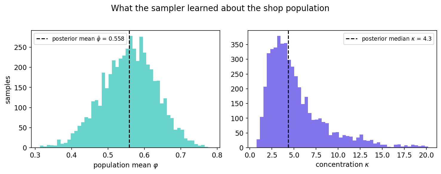
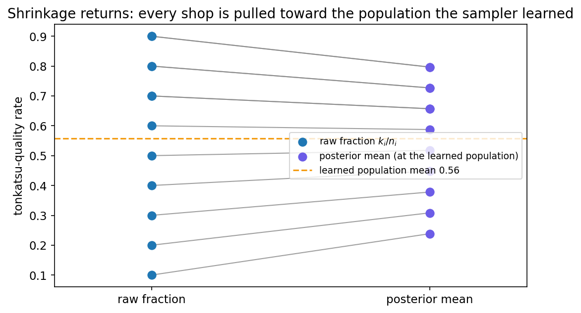
The predictive probability that a brand-new shop’s next rating is good is just the population mean $\varphi$ — the model has learned a prior it can apply to a shop it has never visited, which is the whole point of the hierarchy. And the hierarchy pays its other dividend too: plug the learned population back into each shop’s conjugate posterior, and every shop’s estimate is shrunk toward the population mean — Chapter 12’s partial pooling, now with a population the sampler discovered rather than one we assumed:
Is it converged? (a practical aside)
We discarded the first 1000 sweeps as burn-in and trusted the rest. In practice you would check convergence before trusting any MCMC output — most simply by looking at a trace plot (the parameter plotted against sweep number, as in Chapter 18): after burn-in it should look like stationary noise wobbling around a fixed level, with no drift and no long plateaus stuck in one place. Here is this very sampler’s $\varphi$ trace, with the discarded burn-in shaded:
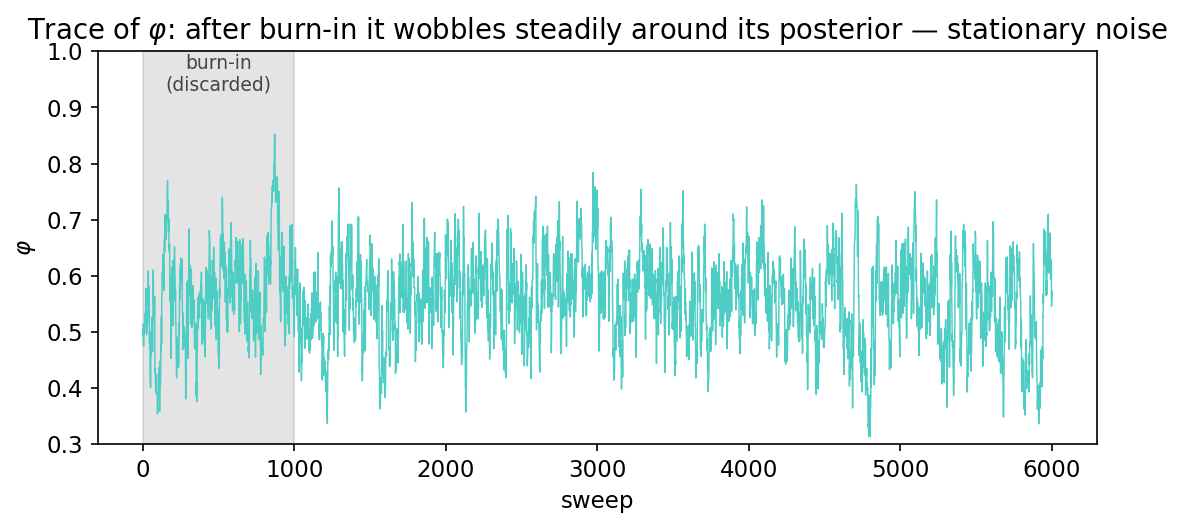
Running the sampler from a few different starts and checking they agree is the multi-chain version of the same idea. We keep it informal here (“run long, discard the first chunk”); formal diagnostics are a topic of their own.
In GenJAX
The hybrid sampler maps cleanly onto GenJAX primitives, and it is worth seeing the split: the Gibbs step is a direct draw from a beta generative model, while the Metropolis step scores the collapsed marginal — there is no joint trace to assess here, because we removed the $\theta_i$ from the population update by integrating them out.
| |
(The Monte Carlo assignment asks you to assemble this same chain in a slightly different way — keeping the $\theta_i$ explicit in the score, and adding a prior on $\kappa$. The mechanism you’ve built here is what it’s testing; the bookkeeping is what it adds.)
Closing the Loop
Step back and see the whole arc. Chapter 13 handed you a Markov chain and you found where it settles. Chapter 15 used a chain to model the wandering of memory. Then Chapter 16 taught estimation by sampling, Chapter 17 made the samples track a moving target, and Chapter 18 ran Chapter 13 backwards — designing a chain to hit a target of our choosing. This chapter cashed it all in twice over: a person, run as a Markov chain, reveals the shape of a concept in their head; and a hybrid Gibbs-Metropolis chain learns the hidden population behind a pile of bento ratings. The walk you first used to model a mind is the same tool, now pointed wherever a posterior is too hard to compute by hand — which is to say, almost everywhere.
The whole toolkit also maps, method for method, onto the GenJAX primitives you’ve been collecting since Tutorial 2 — each classical algorithm is a short composition of them:
| Classical method | GenJAX surface |
|---|---|
| basic Monte Carlo | model.simulate(key, args) + vmap over keys |
| rejection sampling | simulate, keep the draws that match the condition |
| importance sampling | model.importance(key, constraint, args) → (trace, log_weight) |
| particle filter | weight (importance) → resample (categorical) → propagate (simulate) per observation |
| MCMC (Metropolis–Hastings) | assemble from model.assess — score, ratio, accept/reject |
| Gibbs step (conjugate) | a direct beta(...) generative draw |
Why this still matters in 2026
You will rarely hand-write an acceptance ratio again — but the sample → score → reweight-or-accept loop you built in these chapters did not go away. It acquired a learned proposal. A diffusion model is, at heart, a learned reverse-MCMC: a chain trained to walk noise back to data. RLHF samples from a policy and reweights by a reward — likelihood weighting with a learned likelihood. Best-of-$N$ sampling from a language model is importance sampling with a verifier as the weight. The mechanics in these four chapters are the conceptual core of how today’s models are trained, steered, and aligned.
What you can do now
You understand MCMC with People — that a person choosing between options is a Metropolis accept step, so the chain of their choices converges to the prior in their head. You can build a hybrid Gibbs–Metropolis sampler for a hierarchical Beta-Binomial model: Gibbs the per-unit rates from their conjugate Beta conditionals, collapse the rates out via the Beta-Binomial marginal, and Metropolis the population $(\varphi, \kappa)$ — reparametrized to mean and (log-)concentration — by a marginal-likelihood ratio. You know why each step is valid (conjugacy; symmetric proposals; flat priors; kernel composition) and how to read off a predictive from the learned population.
This closes Tutorial 3’s sampling arc. The tools here — Monte Carlo, importance sampling, MCMC — are the computational engine under nearly all modern Bayesian modeling.
Glossary: Markov chain Monte Carlo, Gibbs sampling, Metropolis–Hastings, MCMC with People, conjugate prior, concentration parameter.
Exercises
Try it yourself
- All-alike shops. Replace the data so every shop reads 6/10. Re-run the sampler. What happens to the posterior over $\kappa$ — does the concentration go up or down, and why? (Think about what “all shops alike” says about the spread.) What does this suggest about why a prior on $\kappa$ might be useful when data are very homogeneous?
- Read off a prediction. Using the collected
phis, report the posterior mean and a rough 90% interval for $\varphi$ (the 5th and 95th percentiles). In one sentence, what would you tell Chibany about a brand-new, unrated shop? - Watch the chain. Plot (or print every 200th value of) the trace of $\varphi$ across sweeps. Does it look like stationary noise after burn-in? Now start the chain at $\varphi = 0.05$ instead of $0.5$ — how many sweeps until it forgets that bad start?
A companion notebook works through all of this interactively:
📓 Open in Colab: 19_sampling_the_mind.ipynb
References
- Kemp, C., Perfors, A., & Tenenbaum, J. B. (2007). Learning overhypotheses with hierarchical Bayesian models. Developmental Science, 10(3), 307–321. https://doi.org/10.1111/j.1467-7687.2007.00585.x
- Sanborn, A. N., & Griffiths, T. L. (2007). Markov chain Monte Carlo with people. In Advances in Neural Information Processing Systems, 20 (pp. 1265–1272). https://papers.nips.cc/paper_files/paper/2007/hash/89d4402dc03d3b7318bbac10203034ab-Abstract.html
Special thanks to JPPCA for their generous support of this tutorial series.